library(RwR)
library(ggplot2)
library(tibble)
library(broom)
library(splines)
library(dplyr)
library(glmnet)7 Regression modeling
\[ \DeclareMathOperator*{\argmin}{arg\,min} \DeclareMathOperator*{\argmax}{arg\,max} \]
Warning
This chapter is still a draft and minor changes and corrections can be made without notice.
This chapter deals with a some general problems and questions related to regression modeling and the practical process of data analysis. Some of the general considerations apply to statistics and data analysis in a broad sense, but to keep focus, data analysis is treated in the framework of regression models only.
In the first part of the chapter we position linear and generalized linear models from within a more general framework. This makes it possible to formulate some of the central objectives in regression analysis without relying on specific model assumptions. This also allow us to pinpoint some benefits of the (generalized) linear models over more unstructured model classes.
The chapter concludes in Section 7.3 by introducing basis expansion techniques to capture nonlinear relations within the framework of the (generalized) linear models. The techniques are illustrated by a spline basis expansion of the relation between claim size and insurance sum in the fire insurance example and the modeling of birth weight.
7.1 Outline and prerequisites
The chapter primarily relies on the following four R packages.
7.2 General regression models
There exist a multitude of regression models beyond the linear regression model. The generalized linear models in Chapter 5 are examples. We might lump them all together under the umbrella term nonlinear regression, but that would be a mistake. They serve many different purposes and come in many different shapes and sizes. Some nonlinear regression models focus specifically on nonlinear relations between the outcome and the predictors, while still modeling the conditional expectation of the outcome. Other nonlinear models focus on other targets than the conditional expectation, e.g., the conditional median or other conditional quantiles. Some nonlinear models are used for the sole purpose of producing accurate predictions, while other nonlinear models are used to provide insight on the precise relation between a particular predictor and the outcome.
This book covers linear models and various nonlinear generalizations, whose primary purpose is to explicitly capture relations between individual predictors and the outcome. The generalized linear models covered in Chapter 5 rely on simple linear predictors1 and target the conditional expectations—with one particular form of nonlinearity transforming the linear predictor to the mean value scale. Additionally, and equally important, generalized linear models allow us to model variance heterogeneity, which has consequences for the estimation methodology as well as the statistical inference. In Chapter 11 the outcome is a survival time2 and the target is the conditional hazard function of a survival distribution. One particular class of such survival regression models are models of the conditional expectation of the log-survival time, but most survival models are not directly targeting a conditional expectation. Still, the predictors enter into the conditional survival distribution via a linear predictor.
1 A linear predictor \(\eta = X^T \beta\) is just about the simplest way to encode how the outcome depends on the coordinates of the predictor vector \(X\).
2 Or more generally a time-to-event. That is, the outcome is non-negative, and the outcome distribution models how long time it takes before a particular event occurs.
It is common to refer to the regression models covered in this book as interpretable, but we should be careful about this term. Many of the models might still be difficult to decode for humans. What they share, however, is a clean mathematical characterization of how the outcome distribution depends on any given predictor, a well developed estimation machinery and a well understood statistical inference theory. The latter being particularly important if we want to investigate and document if and how much the outcome depends on a particular predictor. And combined with nonlinear basis expansions, as covered in this chapter, these models can often perform remarkably well in practice, meaning that they can provide good predictive performance and fit data well.
In this chapter we will first treat some general aspects of regression modeling without assuming neither the linear model assumptions A1, A2, A3, nor the generalized linear modeling assumptions GA1, GA2, GA3, but for clarity, the modeling target will remain the conditional expectation throughout the chapter.
Definition 7.1 Let \(X \in \mathbb{R}^p\) and \(Y \in \mathbb{R}\) be random variables and suppose that \(\mathbf{E}(|Y|) < \infty\). The regression function \(m : \mathbb{R}^p \to \mathbb{R}\) is defined by \[ m(x) = \mathbf{E}(Y \mid X = x). \tag{7.1}\]
The regression function \(m\) is in general only uniquely defined almost surely w.r.t. to the distribution of \(X\). Though if it has a continuous version, that version is unique on the support of \(X\). In most applications it is reasonable to assume that \(m\) is continuous and thus a well defined function on the support of \(X\).
A general regression model is a set \(\mathcal{M}\) of regression functions. That is, \[ \mathcal{M} \subseteq \{ m \mid m : \mathbb{R}^p \to \mathbb{R} \}. \] We see that the linearity assumption A1 can be expressed in terms of the regression function as \[ m(x) = x^T \beta, \] which means that the corresponding linear regression model can be expressed as \[ \mathcal{M}_{\mathrm{linear}} = \{ x \mapsto x^T \beta \mid \beta \in \mathbb{R}^p \}. \] The linear regression model is parametrized by the parameter \(\beta\) belonging to the parameter set \(\mathbb{R}^p\).
Most regression models are parametrized by a parameter, abstractly denoted \(\theta \in \Theta\), and we then write the model as \[ \mathcal{M} = \{m_\theta \mid \theta \in \Theta \}. \]
Example 7.1 (Logistic function) A simple classical example is the logistic function for \(p = 1\): \[ m_{\theta}(x) = \alpha + \frac{\beta - \alpha}{1 + e^{(\gamma - x)/\sigma}} \tag{7.2}\] The parameter \(\theta = (\alpha, \beta, \gamma, \sigma)\) is \(4\)-dimensional and the parameter set is \(\Theta = \mathbb{R}^4\). The S-shaped graph of a logistic function can, for instance, model the relation between a dosage (\(x\)) and a continuous outcome (\(y\)).
Example 7.2 (Generalized linear models) With \(\mu : \mathbb{R} \to \mathbb{R}\) any mean value function, a generalized linear model is given by the class of regression functions \[ m_\beta(x) = \mu(x^T \beta), \qquad \beta \in \mathbb{R}^p. \] That is,
\[ \mathcal{M}_{\mathrm{glm}} = \{ x \mapsto \mu(x^T \beta) \mid \beta \in \mathbb{R}^p \} \] with parameter set \(\Theta = \mathbb{R}^p\). We usually regard \(\mu\) as a fixed function and different choices of \(\mu\) then give different models indexed by \(\mu\).
Example 7.3 (Neural networks) The widely used neural networks are flexible regression models that can be perceived as a (substantial) extension of generalized linear models.
We first describe a neural network with a single hidden layer. It is given in terms of two (nonlinear) functions \[
\mu, h: \mathbb{R} \to \mathbb{R}.
\] With \(\mathbf{B}\) a real \(p \times q\) matrix, \(\beta \in \mathbb{R}^{q}\) and \(\alpha \in \mathbb{R}\) we then define the regression function \[
m_{\mathbf{B}, \alpha, \beta} (x) = \mu(\alpha + h(x^T \mathbf{B}) \beta)
\] parametrized by \((\mathbf{B}, \alpha, \beta)\). The convention above is that \(h\) is applied coordinatewisely to the \(q\)-dimensional (row)-vector \(x^T \mathbf{B}\). The mapping \[
x \mapsto h(x^T \mathbf{B})
\] from \(\mathbb{R}^p\) to \(\mathbb{R}^q\) is the input layer, while the mapping
\[
z \mapsto \mu(\alpha + z \beta)
\] from \(\mathbb{R}^q\) to \(\mathbb{R}\) is the output layer. The coordinates of the vector \(h(x^T \mathbf{B})\) are known as the hidden nodes of the network. Generalized linear models can be seen as neural networks with no hidden layers.
The functions \(h\) and \(\mu\) are known as activation functions in the literature on neural networks.
The matrix \(\mathbf{B}\) parametrizes the input layer, while the number \(\alpha\) and the vector \(\beta\) parametrize the output layer. The resulting model \[ \mathcal{M}_{\mathrm{nn}} = \{m_{\mathbf{B}, \alpha, \beta} \mid (\mathbf{B}, \alpha, \beta) \in \mathbb{R}^{p \times q} \times \mathbb{R} \times \mathbb{R}^q \} \] is parametrized by \(\Theta = \mathbb{R}^{p \times q} \times \mathbb{R} \times \mathbb{R}^q\).
To define neural networks with multiple hidden layers, we introduce the notation \[ L_{\alpha, \mathbf{B}}^{h} (x) = h(\alpha + x^T \mathbf{B}) \] for an activation function \(h\), a \(p \times q\) matrix \(\mathbf{B}\) and a vector \(\alpha \in \mathbb{R}^q\). Then \(L_{\alpha, \mathbf{B}}^h : \mathbb{R}^p \to \mathbb{R}^q\) and it represents a single layer in a neural network. Using this notation we can write the single hidden layer neural network regression function above as a composition of two such maps: \[ m_{\mathbf{B}, \alpha, \beta} = L_{\alpha, \beta}^\mu \circ L_{0, \mathbf{B}}^{h} \]
A general neural network with \(k\) hidden layers can be defined as \[ \begin{align*} m_{\alpha_1, \mathbf{B}_1, \ldots, \alpha_k, \mathbf{B}_k, \alpha, \beta} %& = \mu(h_k( \cdots ( h_2(h_1(x^T \mathbf{B}_1)\mathbf{B}_2 + \beta_2) \cdots \mathbf{B}_k) + \beta_k)\beta + \beta_0) \\ & = L_{\alpha, \beta}^\mu \circ L_{\alpha_k, \mathbf{B}_k}^{h_k} \circ \ldots \circ L_{\alpha_1, \mathbf{B}_1}^{h_1} \end{align*} \] The model is parametrized by \((\alpha_1, \mathbf{B}_1, \ldots, \alpha_k, \mathbf{B}_k, \alpha, \beta)\) where \(\mathbf{B}_{j}\) is a \(p_{j-1} \times p_j\) real matrix (\(p_0 = p\)), \(\alpha_j \in \mathbb{R}^{p_j}\), \(\beta \in \mathbb{R}^{p_k}\) and \(\alpha \in \mathbb{R}\).
It is quite common to use the same activation function for all layers, that is, \(h_1 = h_2 = \ldots = h_k = \mu\). A couple of standard choices are: \[ \begin{align*} \mu(\eta) & = (1 + e^{-\eta})^{-1} \qquad \mathrm{(logistic)} \\ \mu(\eta) & = \log(1 + e^\eta) \qquad \ \mathrm{(softplus)} \\ \mu(\eta) & = \max(0, \eta) \qquad \ \ \ \mathrm{(ReLU)}. \end{align*} \]
The four parameter logistic function model above is an example of a neural network with \(p = q = 1\) and activation function being the logistic function.
Even though the parameter space of a neural network can be very large—in particular for deep neural networks with many hidden layers—the parameter space is formally a finite dimensional space. We might want to choose a model \(\mathcal{M}\) that is even larger, e.g., the set of all continuous functions, the set of all Lipschitz functions, or the set of all smooth functions. These sets cannot be parametrized in a nice way by a finite dimensional parameter3, and we call the corresponding regression models nonparametric.
3 More precisely, they are not finite dimensional differentiable manifolds.
There are substantial theoretical differences between trying to estimate a regression function in a parametric model or in a nonparametric model. From a practical perspective, though, the transition from small parametric models to nonparametric models via large parametric models is much more gradual. We will not deal with estimation methods or theory that are explicitly nonparametric, but it can be conceptually advantageous to define and discuss the purposes and objectives of a regression analysis in a nonparametric way. Doing so, we will be able to define our aims clearly without reference to a particular parametric model—even though we eventually, in this book, develop solutions in terms of specific parametric models.
7.2.1 Nonlinear least squares estimation
The most widely used estimator of the regression function is the least squares estimator minimizing the squared error loss. With a model \(\mathcal{M}\) and observations \((X_1, Y_1), \ldots, (X_n, Y_n)\) it is formally defined as \[ \hat{m} = \argmin_{m \in \mathcal{M}} \sum_{i=1}^n (Y_i - m(X_i))^2. \tag{7.3}\] If the model is parametrized by \(\theta \in \Theta\), we can formulate the estimator in terms of estimating \(\theta\) \[ \hat{\theta} = \argmin_{\theta \in \Theta} \sum_{i=1}^n (Y_i - m_{\theta}(X_i))^2. \tag{7.4}\]
Example 7.4 (Logistic model of birth weight) Recall that the relation between birth weight and gestational age appeared roughly \(S\)-shaped in Figure 3.6. To demonstrate fitting a nonlinear regression function by least squares estimation, we therefore attempt to fit the four-parameter logistic curve from Example 7.1. This is done using the nls() function (nonlinear least squares) and the SSfpl() function—a so-called self starting four parameter logistic model.
Code
data("birth_weight")
birth_weight <- filter(
  birth_weight,
  weight > 32,
  length > 10 & length < 99,
  gestationalAge > 18
) |>
  na.omit() |>
  select(- c(interviewWeek, fetalDeath))

binScale <- scale_fill_continuous(
  breaks = c(1, 10, 100, 1000),
  low = "gray80",
  high = "black",
  trans = "log",
  guide = "none"
)
Code
birth_weight_nls <- nls(
    weight ~ SSfpl(gestationalAge, alpha, beta, gamma, sigma),
    data = birth_weight
    )
tidy(birth_weight_nls)
# A tibble: 4 × 5
term estimate std.error statistic p.value
<chr> <dbl> <dbl> <dbl> <dbl>
1 alpha 1463. 112. 13.1 4.98e-39
2 beta 4033. 32.6 124. 0
3 gamma 35.1 0.241 146. 0
4 sigma 2.72 0.174 15.6 2.75e-54The table above shows the four parameter estimates.
Code
birth_weight_diag <- augment(birth_weight_nls)
p1 <- ggplot(birth_weight_diag, aes(x = as.factor(gestationalAge), y = weight)) +
  geom_boxplot(fill = gray(0.8), outlier.alpha = 0.1) +
  geom_line(aes(y = .fitted, group = 1), color = "blue", linewidth = 1) +
  xlab("Gestational age")
p2 <- ggplot(birth_weight_diag, aes(.fitted, .resid)) +
    geom_point(alpha = 0.1) + geom_smooth(linewidth =  1, fill = "blue") +
    ylab("residuals") + xlab("fitted")
gridExtra::grid.arrange(p1, p2, ncol = 2)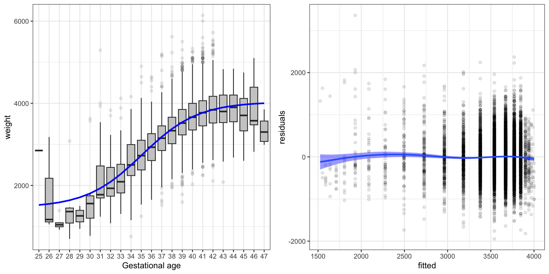
What is most interesting is to compare the fitted model with the data, and Figure 7.1 shows that the model is a reasonably good fit.
Even though Example 7.4 makes it look like nonlinear least squares estimation is as simple as linear least squares, there are several practical issues with the formal definitions of \(\hat{m}\) and \(\hat{\theta}\). Fitting the simple, four parameter logistic curve in Example 7.4 is a fairly easy problem, and the point of the “self starting” model function is that it automatically finds good starting values for the numerical optimization algorithm.
In general, there may first of all be no global minimizer of the sum of squares or there may be many. Second, it may be practically impossible to compute any such global minimizer unless \(\mathcal{M}\) is particularly nice, e.g., \(\mathcal{M} = \mathcal{M}_{\mathrm{linear}}\) as in Theorem 2.1. Third, even if we could compute \(\hat{m}\) it might not be a good estimator if \(\mathcal{M}\) is very large relative to the sample size \(n\).
Many practical estimation algorithms do not attempt to literally compute \(\hat{m}\) or \(\hat{\theta}\) as defined by (7.3) and (7.4), respectively. Typically, they iteratively find and improve candidate regression functions in the model—using the squared error loss as guide rather than trying to drive it to its minimal value.
When using regression models in practice, as well as when we analyze theoretical properties of regression models, it is crucial to understand the difference between literally computing a (unique) minimizer by Equation 7.4 and computing somehow4 a \(\hat{\theta}\) that makes \(m_{\hat{\theta}}\) have a relatively small squared error loss. The latter situation is common for nonlinear regression models, in which case it becomes very difficult to say much about the sampling distribution of \(\hat{\theta}\) or \(m_{\hat{\theta}}\). This, in turn, makes statistical inference difficult.
4 Most numerical optimization algorithms will at best find a local minimizer unless the minimization problem is convex. This fact is compounded by overparametrization of many nonlinear regression models. That is, \[\theta \mapsto (m_\theta(X_i))_{i=1,\ldots,n}\] is non-injective.
Additionally, for a flexible model, \(\hat{m}\) given by Equation 7.3—or obtained by an algorithm that just drives the squared error loss small—often overfits the data. This means that the model adapts so well to the particular data that \(\hat{m}\) actually becomes a bad estimator of \(m\). We can try to combat overfitting by several different methods, e.g., by explicitly restricting the model space to an increasing sequence of \(n\)-dependent subsets \[ \mathcal{M}_1 \subseteq \mathcal{M}_2 \subseteq \ldots \subseteq \mathcal{M}_n \subseteq \ldots \subseteq \mathcal{M} \] and compute \(\hat{m}^n \in \mathcal{M}_n\) for a dataset of size \(n\).
For sufficiently flexible models \(\mathcal{M}\), e.g., models containing all degree \(n\) polynomials, there is a subset \(\mathcal{M}_0 \subseteq \mathcal{M}\) such that for all \(m \in \mathcal{M}_0\), \(m(X_i) = Y_i\) for all \(i = 1, \ldots, n\). All regression functions in \(\mathcal{M}_0\) are said to interpolate the data perfectly, and they all achieve the globally minimal squared error loss of \(0\).
A related, and widely used, way to regularize the estimation problem is via a penalty function \[
\mathrm{pen} : \mathcal{M} \to \mathbb{R}.
\] Optimization algorithms will then (try to) compute
\[
\hat{m}^{\lambda_n} = \argmin_{m \in \mathcal{M}} \sum_{i=1}^n (Y_i - m(X_i))^2 + \lambda_n \mathrm{pen}(m)
\tag{7.5}\] for an \(n\)-dependent parameter \(\lambda_n > 0\) controlling the tradeoff between the squared error loss and the penalty term. Typically, \(\lambda_n \to 0\) for \(n \to \infty\) so that the regularization has less and less impact on the estimator as the sample size increases. Section 7.3 demonstrates by example the use of penalization within the framework of a linear model, where the penalization is used to control the fluctuations of nonlinear interaction terms.
We can interpret the term \(\lambda_n \mathrm{pen}(m)\) as an inductive bias, where we bias the estimator toward small values of \(\mathrm{pen}(m)\). Another way to introduce an inductive bias is by early stopping. If we start the optimization algorithm in a particular subset \(\mathcal{M}_0\) and then stop it before convergence, the result is implicitly biased toward models in \(\mathcal{M}_0\). An algorithm could implement early stopping by monitoring the squared error loss on an independent dataset and stop when that error does not improve anymore. Similarly, the parameter \(\lambda_n\) could be selected by minimizing the squared error loss on an independent dataset over a range of possible values of \(\lambda_n\).
We use inductive bias to mean a model assumption or algorithmic constraint that stear the estimator in a particular direction. The concept is philosophically close to a Bayesian prior, and Bayesian statistics offers a principled way to transform prior beliefs to inductive biases. The folklore interpretation of the No Free Lunch theorem is that we cannot estimate \(m\) to generalize beyond data without some inductive bias.
For a majority of this book we consider parametrized models and loss functions that are nice enough for the estimators we consider to actually be global minimizers, such that \(\hat{\theta}\) is really given by (7.4). The least squares estimator in \(\mathcal{M}_{\mathrm{linear}}\), as treated in detail in Chapter 2, stands out as having a particularly well understood theory, which we can leverage for practical statistical data analysis. When estimation is done by running complicated algorithms on data, so that the estimator has no simple analytic representation, e.g., as the solution of an equation, we cannot obtain a similarly simple theory. This does not make such estimators bad, but we then have to reach out for different ways of doing statistical inference.
We will demonstrate in this chapter how to articulate questions of interest in terms of general regression models, and we will show how we can capture those questions within nice parametric model classes, such as linear and generalized linear models, and how the statistical theory of those models then provide tools for answering the questions of interest.
7.2.2 Regression modeling objectives
As discussed at some length in Chapter 1, one purpose of estimating the regression function \(m\) is to use \(\hat{m}\) to make predictions about \(Y\) from observation of \(X\). This is the primary focus in most of the machine learning literature. Though we will cover this aspect in Chapter 8—where we discuss quantification and optimization of predictive strength of a model—we also deal at length with other objectives.
One main objective we consider is:
In this section we focus for clarity on how \(m\) depends on a single coordinate of the predictor vector. Similar questions can, of course, be formulated for any group of coordinates, and this is how we would deal with categorical predictors or when investigating interactions.
Does \(m\) depend on \(x_j\)?
To formulate this precisely, let \(x_{-j} = (x_1, \ldots, x_{j-1}, x_{j+1}, \ldots, x_p)^T\) denote the \((p-1)\)-dimensional vector with the \(j\)-th coordinate removed from \(x\), and let \[ m_{-j}(x_{-j}) = \mathbf{E}(Y \mid X_{-j} = x_{-j}) \] denote the regression function based on the \(X_{-j}\)-predictors only. We can then formulate the hypothesis \[ H_0: \mathbf{E}(Y \mid X) = m_{-j}(X_{-j}). \tag{7.6}\] This hypothesis means that \(m\) does not depend on the \(j\)-th coordinate of the predictor, and it is an example of a conditional (mean) independence hypothesis. We discuss below how this hypothesis is expressed in generalized linear models and how we test the hypothesis.
Another main objective we consider is:
Quantify how much \(m\) depends on a particular coordinate \(x_j\).
Obviously, this objective is closely related to the hypothesis above—any sensible quantification should show that \(m\) does not depend on \(x_j\) if \(H_0\) is true. Additionally, such a quantification is naturally tied together with the development of a test statistic of \(H_0\). Testing \(H_0\) is, however, a simpler problem, and the challenge is to develop easily interpretable quantifications that are simultaneously easy to estimate. The regression modeling frameworks we consider will have some natural ways of quantifying such conditional associations.
To aid the general discussion of the two objectives above, we introduce partial dependence functions and partial errors below. To ease notation we will use the convention that \[ m(x_j, x_{-j}) = m((x_1, \ldots, x_{j-1}, x_j, x_{j+1}, \ldots, x_{p})^T), \] where \(m(x_j, x_{-j})\) is simply a shorthand notation for the right hand side above. Recall that \(m(x) = \mathbf{E}(Y \mid X = x)\) denotes the joint regression function of \(Y\) on \(X\) with the additive error defined as \[ \varepsilon = Y - m(X). \]
Definition 7.2 Let \[ m_{-j}(x_{-j}) = \mathbf{E}(Y \mid X_{-j} = x_{-j}) \] denote the regression function of \(Y\) given \(X_{-j}\) excluding the \(j\)-th coordinate of \(X\). The \(j\)-th partial error is defined as \[ \varepsilon_{-j} = Y - m_{-j}(X_{-j}). \tag{7.7}\]
Note that the tower property of conditional expectations imply the identity \[ m_{-j}(x_{-j}) = \mathbf{E}( m(X_j, x_{-j}) \mid X_{-j} = x_{-j}), \] which relates \(m_{-j}\) to \(m\).
It is generally difficult for a multivariate function \(m\) to understand how it depends on a single coordinate. Therefore we introduce a univariate function that summarizes this dependence by averaging over all other coordinates.
Definition 7.3 The partial dependence function \(m_j : \mathbb{R} \to \mathbb{R}\) for the \(j\)-th coordinate is \[ m_j(x_j) = \mathbf{E}(m(x_j, X_{-j})) = \mathbf{E}(\mathbf{E}(Y \mid X_j = x_j, X_{-j})). \tag{7.8}\]
The partial dependence function is also known as the adjusted regression function. Note that in its definition we integrate out over the marginal distribution of \(X_{-j}\) and not the conditional distribution of \(X_{-j}\) given \(X_{j} = x_j\).
Example 7.5 If \(m(x) = x^T \beta\) is linear we find that
\[
m_{-j}(x_{-j}) = x_{-j}^T \beta_{-j} + \beta_j \mathbf{E}(X_j \mid X_{-j} = x_{-j})
= x_{-j}^T \beta_{-j} + \beta_j r_j(x_{-j}).
\] where \(r_j(x_{-j}) \coloneqq \mathbf{E}(X_j \mid X_{-j} = x_{-j})\) only depends on the distribution of \(X\). We get that
\[
m(X) - m_{-j}(X_{-j}) = \beta_j(X_j - r_j(X_{-j})),
\] which is almost surely zero if either \(\beta_j = 0\) or \(X_j = r_j(X_{-j})\). Ruling out situations of perfect collinearity5 among the predictors we see that \(H_0\) given by Equation 7.6 is equivalent to \[
H_0: \beta_j = 0
\] for the linear model. The \(F\)-test defined by Equation 2.11 can thus be used to formally test \(H_0\). Note that the \(F\)-test statistic generalizes straightforwardly to testing if \(m\) does not depend on a group of predictors.
5 That \(X_j\) is almost surely not equal to a function of \(X_{-j}\) can be expressed as \(\mathbf{V}(X_j - r_j(X_{-j})) > 0\).
Moreover, since \[ \varepsilon_{-j} = Y - m(X) + m(X) - m_{-j}(X_{-j}) = \varepsilon + \beta_j(X_j - r_j(X_{-j})), \] we find that \[ \mathrm{cov}(\varepsilon_{-j}, X_j) = \beta_j \mathbf{V}(X_j - r_j(X_{-j})), \] and the \(\beta_j\) parameter can be recovered as \[ \beta_j = \frac{ \mathrm{cov}(\varepsilon_{-j}, X_j) }{\mathbf{V}(X_j - r_j(X_{-j}))}. \] Finally, the partial dependence function is \[ m_j(x_j) = \beta_j x_j + \mathbf{E}(X_{-j})^T \beta_{-j}, \] which is affine with slope \(\beta_j\), and it is constant if and only if \(\beta_j = 0\).
For the linear model above, all of the quantities \(m_j\), \(m(x) - m_{-j}(x_{-j})\) and \(\mathrm{cov}(\varepsilon_{-j}, X_j)\) were linked directly to the coefficient \(\beta_j\). We now show a general result linking the hypothesis \(H_0\) to the partial dependence function and the partial error.
Proposition 7.1 If the regression function \(m(x) = \mathbf{E}(Y \mid X = x)\) does not depend on \(x_j\) then
- The partial dependence function \(m_{j}\) is constant.
- \(m_{-j}(x_{-j}) = m(x_j, x_{-j})\) for any \(x_j\).
- \(\mathrm{cov}(\varepsilon_{-j}, h(X_j)) = 0\) for any function \(h\) such that \(h(X_j)\) has finite second moment.
Proof. It follows directly from (7.8) that if \(m\) does not depend on \(x_j\) then \(m_{j}(x_j) = \mathbf{E}(m(X_{-j}))\) is constant.
To prove the second claim we note that if \(m\) does not depend on the \(j\)-th coordinate, \(m(X_j, x_{-j}) = m(x_j, x_{-j})\) for any fixed \(x_j\), whence \[ m_{-j}(x_{-j}) = \mathbf{E}( m(X_j, x_{-j}) \mid X_{-j} = x_{-j}) = m(x_j, x_{-j}). \]
Finally, if \(m\) does not depend on \(x_j\), \(\varepsilon_{-j} = \varepsilon = Y - \mathbf{E}(Y \mid X)\). Whence by the tower property of conditional expections, \[ \begin{align*} \mathrm{cov}(\varepsilon_{-j}, h(X_j)) & = \mathrm{cov}(\varepsilon, h(X_j)) \\ & = \mathbf{E}( \varepsilon h(X_j) ) \\ & = \mathbf{E}( \mathbf{E}(\varepsilon h(X_j) \mid X)) \\ & = \mathbf{E}( \mathbf{E}(\varepsilon \mid X) h(X_j)) = 0, \end{align*} \] where we have used that \(\mathbf{E}(\varepsilon \mid X) = 0\).
There are various procedures, motivated by Proposition 7.1, that are used in practice to better understand how \(m\) depends on a particular predictor. To describe them, let \(\hat{m}\) and \(\hat{m}_{-j}\) denote estimates of \(m\) and \(m_{-j}\), respectively.
- The partial dependence plot is simply a plot of \(\hat{m}_j(x_j)\) against \(x_j\), where \[ \hat{m}_j(x_j) = \frac{1}{n} \sum_{i=1}^n \hat{m}(x_j, X_{i, -j}). \] It is a direct graphical check of whether \(m_j\) is constant.
- For a \(p\)-dimensional model \(\mathcal{M}\) of \(m\) and a \(p_0\) dimensional model \(\mathcal{M}_{-j}\) of \(m_{-j}\), the \(F\)-test statistic is defined as \[ F = \frac{\sum_{i=1}^n (\hat{m}_{-j}(X_{i,-j}) - \hat{m}(X_{i}))^2/(p - p_0)}{\sum_{i=1}^n(Y_i - \hat{m}(X_{i}))^2 / (n - p)}. \tag{7.9}\] It quantifies directly any differences between \(m_{-j}\) and \(m\), though it cannot generally be expected to be \(F\)-distributed under \(H_0\).
- Defining the \(j\)-th partial residuals as \[ \hat{\varepsilon}_{i, -j} = Y_i - \hat{m}_{-j}(X_{-j}), \] we can plot \(\hat{\varepsilon}_{i, -j}\) against \(X_{i,j}\).
- Letting \(\hat{r}_j\) denote an estimate of the regression function \[ r_j(x_{-j}) = \mathbf{E}(X_j \mid X_{-j} = x_{-j}), \] we can also plot the partial residuals \(\hat{\varepsilon}_{i,-j}\) against \(X_{i,j} - \hat{r}_j(X_{i,-j})\). This plot is known as an added variable plot.
The suggested plots of the partial residuals against either the \(j\)-th predictor or its residual are both attempts to visualize dependencies between \(\varepsilon_{-j}\) and \(X_j\). The plots can be used to graphically detect if \(\mathrm{cov}(\varepsilon_{-j}, X_j) = 0\) or not, and we can use them to assess linear modeling assumptions.
We can also use the partial residuals to directly estimate the covariance, either as \[ \widetilde{\mathrm{cov}}_j = \frac{1}{n} \sum_{i=1}^n \hat{\varepsilon}_{i, -j} X_{i,j} \tag{7.10}\] or as \[ \widehat{\mathrm{cov}}_j = \frac{1}{n} \sum_{i=1}^n \hat{\varepsilon}_{i, -j} (X_{i,j} - \hat{r}(X_{i,-j})). \tag{7.11}\]
Both of these covariance estimates quantify deviations from \(H_0\), and in this way indirectly also how much \(m\) depends on the \(j\)-th coordinate. The estimator (7.10) has the advantage that we do not need to estimate the regression function \(r_j\), but it can be severely biased and \(\widehat{\mathrm{cov}}_j\) is preferred in practice.
Example 7.6 For a generalized linear model, \[ m(x) = \mu(x^T\beta), \] and a partial dependence plot is obtained by computing \[ \hat{m}_j(x_j) = \frac{1}{n} \sum_{i=1}^n \mu(x_j \hat{\beta}_j + X_{i,-j}^T \hat{\beta}_{-j}) \] for a range of \(x_j\)-s.
Due to the nonlinear mean value function \(\mu\), the partial dependence function and other constructions, such as the partial error, do not have expressions the simplify as gracefully as for the linear model. The partial dependence function is, for instance, nonlinear in \(x_j\) and its shape depends on the distribution of \(X_{-j}\).
It is, nevertheless, clear that \(m\) does not depend on \(x_j\) if and only if \(\beta_j = 0\), and a test of \(H_0\) given by Equation 7.6 can be carried out using the deviance based test statistics of Definition 5.2.
With the terminology from Chapter 5, the fitted values are denoted \[ \hat{\mu}_i = \hat{m}(X_i) = \mu(X_i^T \hat{\beta}). \] If we exclude the \(j\)-th predictor, the corresponding fitted values become \[ \hat{\mu}_{i, -j} = \hat{m}_{-j}(X_{i, -j}) = \mu(X_{i, -j}^T \hat{\beta}^{(-j)}). \] Note a subtle but important detail: \(\hat{\beta}^{(-j)}\) denotes the estimate of \(\beta_{-j}\) when the model is fitted excluding the \(j\)-th predictor, while \(\hat{\beta}_{-j}\) above denotes the estimate based on data with the \(j\)-th predictor included, but where the \(j\)-th coordinate from the parameter estimate is just removed.
Recalling the quadratic approximation of the deviances from Theorem 4.2, \[ d(Y_i, \hat{\mu}_i) \approx \frac{(Y_i - \hat{\mu}_i)}{\mathcal{V}(\hat{\mu}_i)} \] and the deviance based \(F\)-test statistic of Definition 5.2 can be approximated as \[ \frac{(D_0 - D)/(p - p_0)}{D / (n - p)} \approx \frac{\sum_{i=1}^n \mathcal{V}(\hat{\mu}_i)^{-1}(\hat{\mu}_{i, -j} - \hat{\mu}_i)^2 /(p - p_0) }{\sum_{i=1}^n \mathcal{V}(\hat{\mu}_i)^{-1}(Y_i - \hat{\mu}_i)^2 /(n - p)}, \] which is similar to the generic \(F\)-test statistics in Equation 7.9 except for the standardization of the terms by the variance function.
Similarly, the raw partial residuals are \[ \hat{\varepsilon}_{i,-j} = Y_i - \hat{\mu}_{i,-j}, \] but for generalized linear models we prefer the standardized partial residuals \[ \frac{Y_i - \hat{\mu}_{i,-j}}{\sqrt{\mathcal{V}(\hat{\mu}_{i,-j})}} \] if we want to quantify residual covariation with \(X_j\).
One of the great benefits of linear and generalized linear models is that the hypotheses of fundamental importance, that can be expressed by Equation 7.6 for one or a group of predictor variables, are encoded by linear hypotheses in the parameter space. And we have tools for testing such hypotheses. Deviations are additionally quantified via the \(\beta\)-parameters, or more precisely by how these parameters model the conditional expectation on the scale of the linear predictor. This scale is, on the other hand, also the more cryptic part of interpreting generalized linear models. For a logit-link model, the \(\beta\)-parameters quantify changes on a log-odds ratio scale and not the probability scale. But even if the scale used to measure deviations may be challenging to understand, it is explicit and not obscure.
We should contrast the situation of linear and generalized linear models with that of neural networks. With a single hidden layer, \(m\) does not depend on \(x_j\) if and only if \[ h(x^T \mathbf{B})\beta = \sum_{k} h\left( x_j B_{jk} + \sum_{j' \neq j} x_{j'} B_{j'}k\right) \beta_k \] does not depend on \(x_j\). Obviously, this is the case if \(B_{jk} = 0\) for all \(k\). However, it is also the case even if some \(B_{jk'} \neq 0\) if just \(\beta_{k'} = 0\). The nonlinearity of \(h\) may add additional parameter values that make \(m\) independent of \(x_j\) and adding additional hidden layers does not improve the situation. The upshot is that even though the hypothesis (7.6) can be encoded by certain parameter constraints on the neural network, it cannot be encoded by a suitably nice subset of the parameter space, and its parametrization does not lead to any useful statistical theory for testing (7.6) or quantifying deviations from (7.6).
7.3 Nonlinear basis expansions
One of the most obvious objections to linear and generalized linear models is that they lack flexibility, which may result in model misspecification. That is, models that do not fit the data well. Another objection is that they may lack predictive strength.
We have already seen various techniques in Chapter 2 and Chapter 3 for transforming the raw predictor variables in the dataset, e.g., a marginal log-transformation, the dummy variable encoding of categorical variables and the encoding of interactions among predictors. Exercise 2.1 elaborates further on using variable transformation in combination with the linear model.
In this section we take variable transformation to its natural conclusion by allowing for any transformation of the raw predictors into a, possibly high-dimensional, space \(\mathbb{R}^p\) via a flexible class of functions. Thus with a \(q\)-tuple of raw predictors, we express the regression function within a generalized linear modeling framework as \[ m(x) = \mu\left( \sum_{k=1}^q \sum_{l=1}^{r_k} \beta_{kl} h_{kl}(x_k) \right) \tag{7.12}\] where \(h_{kl}\) are known functions with \(h_{kl}(x_k) \in \mathbb{R}\) and \(\beta_{kl} \in \mathbb{R}\) are free parameters. With \(p = \sum_{k} r_k\) we collect the values \(h_{kl}(x_k)\) into an vector in \(\mathbb{R}^p\). We refer to the functions \(h_{kl}\) as basis functions and Equation 7.12 as a basis function expansion. In the machine learning literature, it is common to refer to the map \[ x \mapsto (h_{kl}(x_k))_{k=1, \ldots, q, l = 1, \ldots, r_k} \] as a feature map and the \(h_{kl}(x_k)\)-s as features. Note that each “raw predictor” might actually itself be a tuple so that interaction effects are captured by the abstract construction above.
Since the transformation of the raw predictors is done as a pre-processing step, prior to any estimation, the notation simply absorbs any such transformation implicitly into the predictor vector. Thus the basis expansion will not appear explicitly in the theoretical formulas—there we will simply have a predictor vector \(X \in \mathbb{R}^p\), irrespectively of how it is computed from the raw predictors. In practice, we will need to specify the basis expansion either by explicitly transforming the predictors, via the formula interface for model specifications or by a third method.
It may be useful to contrast basis expansions with neural networks. With a single hidden layer we can regard the map \[ x \mapsto h(x^T \mathbf{B})_k = h\left( \sum_{j=1}^p x_j B_{jk} \right) \] for \(k = 1, \ldots, q\) as a \(q\)-dimensional basis expansion (or feature map). If \(B_{jk} \neq 0\) for all \(j,k\), all coordinates of \(x\) enter into all coordinates of this hidden layer. All features thus depend on everything. But the main difference is that this map is also fitted to data for a neural network via estimation of \(B\). The “basis expansion” as implemented by a neural network via its hidden layer(s) is therefore data adaptive, but the price paid is that the model space becomes a complicated object. The basis expansions we will consider, with a fixed set of transformations, result in well behaved model spaces, estimation algorithms and statistical procedures, but are perhaps not quite as data adaptive.
We will in the following two sections return to the linear models of insurance claims from Chapter 2 and of birth weight from Chapter 3. In both cases we found a lack of model fit, and in both cases we will demonstrate how basis expansions can solve this problem.
7.3.1 Nonlinear expansions for claims modeling
We found in Section 2.7.1 that the linear model of the insurance claim sizes did not fit the data. Specifically, the mean value specification did not capture the conditional expectation adequately, as the residual plots showed. This could be due to a nonlinear relation between log(claims) and log(sum). To handle nonlinear relations between the outcome and one or more predictors, the predictors (as well as the outcome) can be nonlinearly transformed before they enter into the linear model. Such pre-modeling transformations extend the scope of the linear model considerably. For the insurance data the original variables were already log-transformed, and it is not obvious which other transformation to use.
Code
x <- seq(11, 21, 0.05)
pol <- as_tibble(cbind(x, poly(x, degree = 5)))
long_pol <- tidyr::pivot_longer(pol, cols = !x, names_to = "basis_fct")
p <- ggplot(NULL, aes(x, value, colour = basis_fct)) +
    scale_color_discrete(guide = "none") + xlab("") + ylab("")
p + geom_line(data = long_pol, linewidth = 1)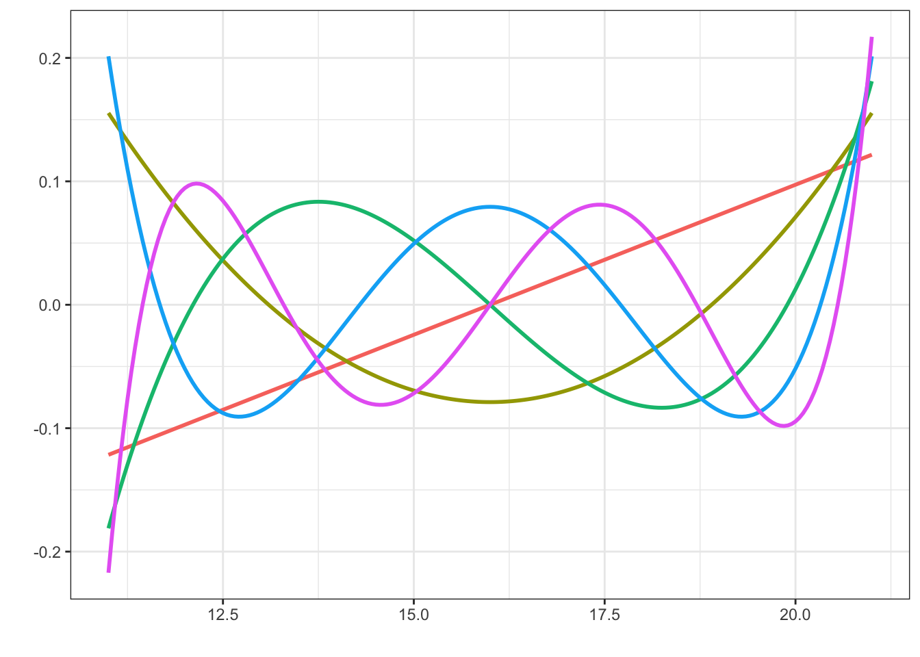
An alternative to data transformations is to use a small but flexible class of basis functions, which can capture the nonlinearity. One possibility is to use low degree polynomials. This can be done by simply including powers of a predictor as additional predictors. [Due to the parsing of formulas in R, powers have to be wrapped into an I()-call, e.g., y ~ x + I(x^2).] Depending on the scale and range of the predictor, this may work just fine. However, raw powers can result in numerical difficulties. An alternative is to use orthogonal polynomials, which are numerically more well behaved.
Figure 7.2 shows an example of an orthogonal basis of degree 5 polynomials on the range 11–21. This corresponds approximately to the range of log(sum), which is a target for basis expansion in the example. What should be noted in Figure 7.2 is that the behavior near the boundary is quite erratic. This is characteristic for polynomial bases. To achieve flexibility in the central part of the range, the polynomials become erratic close to the boundaries. Extrapolation beyond the boundaries cannot be trusted.
An alternative to polynomials is splines. A spline6 is piecewisely a polynomial, and the pieces are joined together in a sufficiently smooth way. The points where the polynomials are joined together are called knots. The flexibility of a spline is determined by the number and placement of the knots and the degree of the polynomials. A degree \(k\) spline is required to be \(k-1\) times continuously differentiable. A degree 3 spline, also known as a cubic spline, is a popular choice, which thus has a continuous (piecewise linear) second derivative.
6 A spline is also a thin and flexible wood or metal strip used for smooth curve drawing.
Code
b_spline <- as_tibble(cbind(x, splines::bs(x, knots = c(14, 18))))
long_b_spline <- tidyr::pivot_longer(b_spline, cols = !x, names_to = "basis_fct")
p + geom_line(data = long_b_spline, linewidth = 1) +
    geom_rug(aes(x = c(11, 14, 18, 21), y = NULL, color = NULL), linewidth = 1)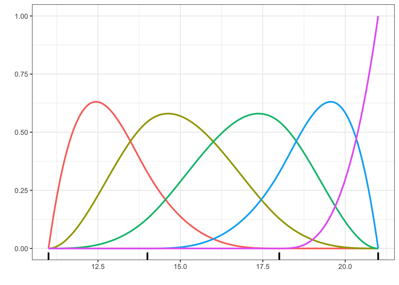
bs() function with two internal knots at 14 and 18 in addition to two boundary knots at 11 and 21.
Figure 7.3 shows a basis of 5 cubic spline functions. They are so-called \(B\)-splines (basis splines). Note that it is impossible to visually detect the knots where the second derivative is non-differentiable. The degree \(k\) \(B\)-spline basis with \(r\) internal knots has \(k + r\) basis functions. The constant function is not included then, and this is precisely what we want when the basis expansion is used in a regression model including an intercept. As seen in Figure 7.3, the \(B\)-spline basis is also somewhat erratic close to the boundary. For a cubic spline, the behavior close to the boundary can be controlled by requiring that the second and third derivatives are \(0\) at the boundary knots. The result is known as a natural cubic spline. The extrapolation (as a spline) of a natural cubic spline beyond the boundary knots is linear.
Due to the restriction on the derivatives of a natural cubic spline, the basis with \(r\) internal knots has \(r + 1\) basis functions. Thus the basis for the natural cubic splines with \(r + 2\) internal knots has the same number of basis functions as the raw cubic \(B\)-spline basis with \(r\) internal knots. This means in practice that, compared to using raw \(B\)-splines with \(r\) internal knots, we can add two internal knots, and thus increase the central flexibility of the model, while retaining its complexity in terms of \(r + 3\) parameters.
Code
n_spline <- as_tibble(cbind(x, splines::ns(x, knots = c(13, 15, 17, 19))))
long_n_spline <- tidyr::pivot_longer(n_spline, cols = !x, names_to = "basis_fct")
p + geom_line(data = long_n_spline, linewidth = 1) +
    geom_rug(aes(x = c(11, 13, 15, 17, 19, 21), y = NULL, color = NULL), linewidth = 1)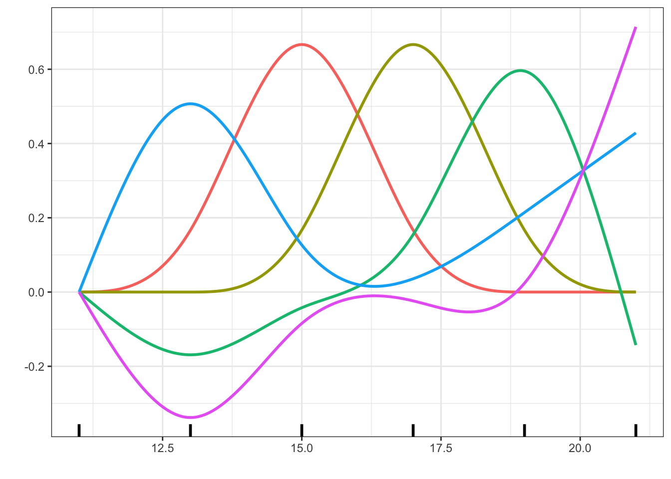
ns() function with internal knots at 13, 15, 17 and 19 in addition to the two boundary knots at 11 and 21.
It is possible to use orthogonal polynomial expansions as well as spline expansions in R together with the lm() function via the functions poly(), bs() and ns(). The latter two are in the splines package, which thus has to be loaded.
We will illustrate the usage of basis expansions for claim size modeling using natural cubic splines of log(sum), of the form
\[ \beta_0 + \beta_1 h_1 + \beta_2 h_2 + \beta_3 h_3 + \beta_4 h_4 + \beta_5 h_5, \] where \(h_1, \ldots, h_5\) are \(B\)-spline basis functions.
Code
ns_log <- function(x) ns(log(x), knots = c(13, 15, 17, 19))
claims_lm_spline_add <- lm(
  log(claims) ~ ns_log(sum) + grp,
  data = claims
)
claims_lm_spline_int <- lm(
  log(claims) ~ ns_log(sum) * grp,
  data = claims
)
When we fit a model using basis expansions the coefficients of individual basis functions are rarely interpretable or of interest. Thus reporting the summary including all the estimated coefficients is not particularly informative. Below we only extract the last lines from the summary to report the residual variance and the \(R^2\) quantities.
Code
glance(claims_lm_spline_add) |>
knitr::kable()| r.squared | adj.r.squared | sigma | statistic | p.value | df | logLik | AIC | BIC | deviance | df.residual | nobs |
|---|---|---|---|---|---|---|---|---|---|---|---|
| 0.06416 | 0.0623 | 1.9185 | 34.509 | 0 | 8 | -8352 | 16724 | 16787 | 14822 | 4027 | 4036 |
Code
glance(claims_lm_spline_int) |>
knitr::kable()| r.squared | adj.r.squared | sigma | statistic | p.value | df | logLik | AIC | BIC | deviance | df.residual | nobs |
|---|---|---|---|---|---|---|---|---|---|---|---|
| 0.07294 | 0.06762 | 1.9131 | 13.724 | 0 | 23 | -8333 | 16716 | 16874 | 14683 | 4012 | 4036 |
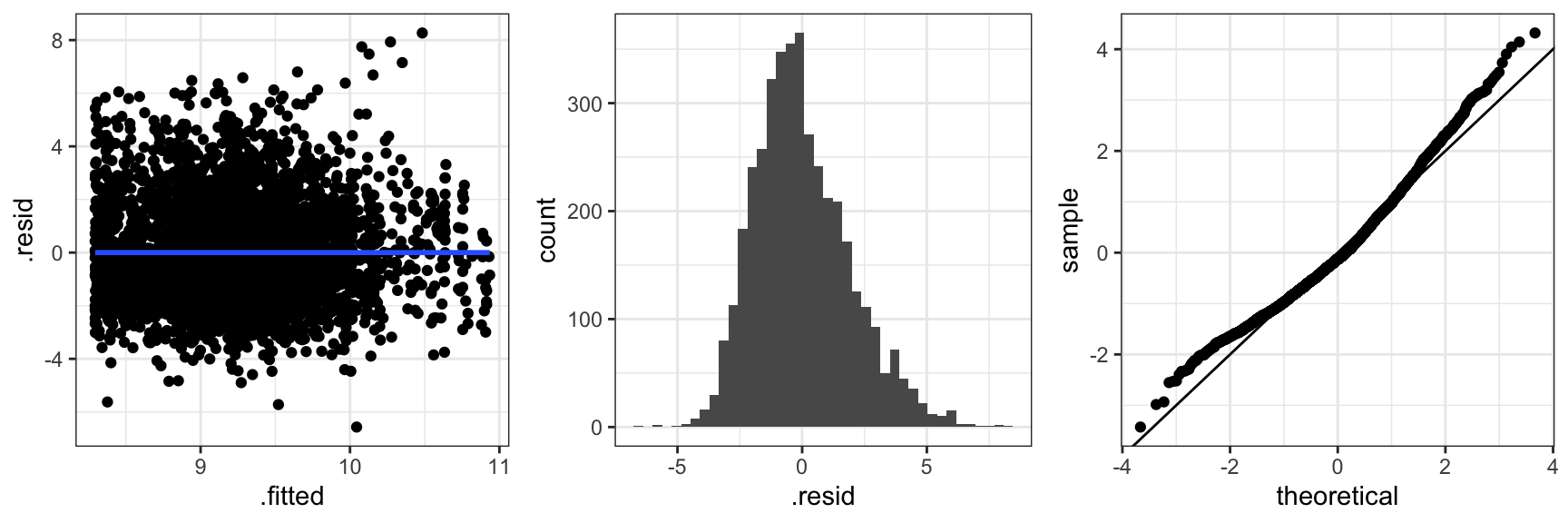
Compared to the additive model without the basis expansion, \(R^2\) (also the adjusted one) is increased a little by the basis expansion. A further increase is observed for the model that includes interactions as well as a basis expansion, and thus gives a unique nonlinear relation between insurance sum and claim size for each trade group. Figure 7.5 shows some diagnostic plots for the additive model, which show that the mean value model is now pretty good, while the residuals are still slightly right skewed. The lack of normality is not a problem for using the sampling distributions to draw inference. However, if we compute prediction intervals, say, then we must account for the skewness in the residual distribution. This can be done by using quantiles for the empirical distribution of the residuals instead of quantiles for the normal distribution.
Code
claims_diag_spline <- augment(claims_lm_spline_add) ## Residuals etc.
gridExtra::grid.arrange(
  ggplot(claims_diag_spline, aes(.fitted, .resid)) + geom_point(alpha = 0.2) + geom_smooth(),
  ggplot(claims_diag_spline, aes(.resid)) + geom_histogram(bins = 40),
  ggplot(claims_diag_spline, aes(sample = .std.resid)) + geom_qq() + geom_abline(),
  ncol = 3
)
Graphical comparisons are typically preferable over parameter comparisons when models involving nonlinear effects and basis expansions are compared.
Code
p0 <- ggplot(
        data = claims,
        aes(sum, claims)
    ) +
    scale_x_log10(
        "Insurance sum (DKK)",
        breaks = 10^c(6, 7, 8),
        labels = c("1M", "10M", "100M")
        ) +
    scale_y_log10(
        "Claim size (DKK)",
        breaks = 10^c(2, 4, 6, 8),
        labels = c("100", "10K", "1M", "100M")
    ) +
    geom_point(alpha = 0.2)
Code
pred_add <- cbind(
    claims,
    exp(predict(claims_lm_spline_add, interval = "confidence"))
)
pred_int <- cbind(
    claims,
    exp(predict(claims_lm_spline_int, interval = "confidence"))
)
p0 <- p0 + facet_wrap(~ grp, ncol = 4) + coord_cartesian(ylim = c(100, 1e6))
p0 + geom_line(aes(y = fit), pred_add, color = "blue", linewidth = 2) +
  geom_ribbon(aes(ymax = upr, ymin = lwr), pred_add, fill = "blue", alpha = 0.2) +
  geom_line(aes(y = fit), pred_int, color = "red", linewidth = 2) +
  geom_ribbon(aes(ymax = upr, ymin = lwr), pred_int, fill = "red", alpha = 0.2)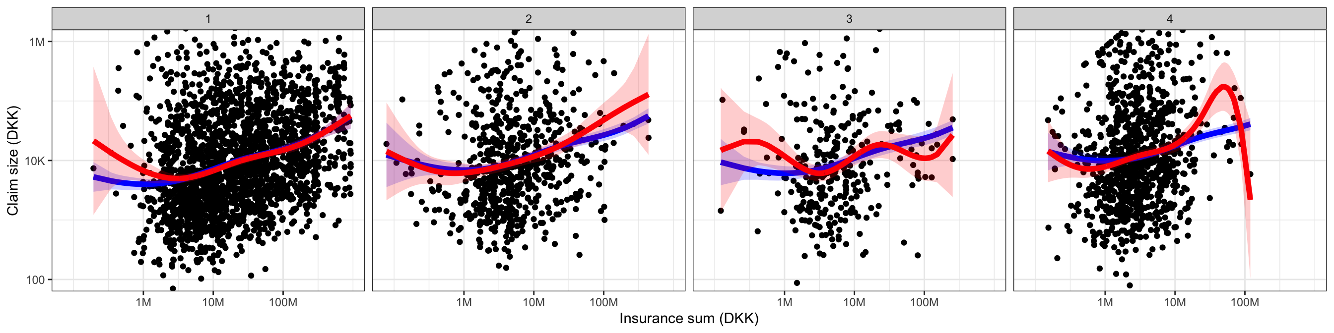
Figure 7.6 shows the fitted models stratified according to trade group. The fitted values were computed using the predict() function in R, which can also give upper and lower confidence bounds on the fitted values. The fitted value for the \(i\)-th observation is \(X_i^T \hat{\beta}\). By Theorem 2.3 a confidence interval for the fitted value can be computed using Equation 2.10 with \(a = X_i\). The confidence intervals reported by predict() for lm objects are computed using this formula, and these are the pointwise confidence bands shown in Figure 7.6. From this figure any gain of the interaction model over the additive model is questionable. The increase of \(R^2\), say, appears to be mostly driven by spurious fluctuations. For trade group 4 the capped claims seem overly influential, and because trade group 3 has relatively few observations the nonlinear fit is poorly determined for this group.
In a final comparison below using \(F\)-tests we first test the hypothesis that the relation is linear in the additive model, and then we test the additive hypothesis when the nonlinear relation is included. The tests formally reject both hypotheses, but the graphical summary in Figure 7.6 suggests that the nonlinear additive model is preferable anyway due to the irregular fluctuations of the interaction model.
Code
claims_lm_add <- lm(
    log(claims) ~ log(sum) + grp,
    data = claims
)
Code
anova(
    claims_lm_add,
    claims_lm_spline_add,
    claims_lm_spline_int
) |> knitr::kable()| Res.Df | RSS | Df | Sum of Sq | F | Pr(>F) |
|---|---|---|---|---|---|
| 4031 | 14902.71 | NA | NA | NA | NA |
| 4027 | 14822.42 | 4 | 80.28605 | 5.484225 | 0.0002115 |
| 4012 | 14683.37 | 15 | 139.04900 | 2.532863 | 0.0009413 |
Introducing a penalty can dampen the spurious fluctuations that arose from the nonlinear basis expansion. We conclude the analysis of the insurance data by illustrating how the penalized least squares fit can be computed, and what effect the penalty has on the least squares solution. First recall that the least squares estimator could have been computed by solving the normal equation directly.
\[
\mathbf{X}^T \mathbf{X} \beta = \mathbf{X}^T \mathbf{Y}.
\] We compute the solution using solve() in R.
Code
X <- model.matrix(claims_lm_spline_int)
y <- model.response(model.frame(claims_lm_spline_int))
XtX <- crossprod(X)     # Faster than but equivalent to t(X) %*% X
Xty <- crossprod(X, y)  # Faster than but equivalent to t(X) %*% y
coef_hat <- solve(XtX, Xty)
# Comparison
range(coef_hat - coefficients(claims_lm_spline_int))
[1] -1.125585e-09 7.045786e-11The result obtained by solving the normal equation directly is up to numerical errors identical to the solution computed using lm(). The R function solve() calls the Fortran routine DGESV from the LAPACK library for solution of linear equations using LU decomposition with partial pivoting (Gaussian elimination with row permutations).
Likewise, we can compute the penalized estimator by solving the corresponding linear equation, which now includes the \(\boldsymbol{\Omega}\) penalty matrix,
\[ \left(\mathbf{X}^T \mathbf{X} + \boldsymbol{\Omega}\right) \beta = \mathbf{X}^T \mathbf{Y}. \] We will do so where we only add a penalty on the coefficients corresponding to the interaction terms in the nonlinear basis expansion. We will use penalty matrices of the form \(\lambda \boldsymbol{\Omega}\) for a fixed matrix \(\boldsymbol{\Omega}\) so that the amount of penalization is controlled by the parameter \(\lambda > 0\).
Code
Omega <- diag(c(rep(0, 9), rep(1, 15)))
coef_hat <- cbind(
    solve(XtX + 0.1 * Omega, Xty),  # Small penalty
    solve(XtX + Omega, Xty),        # Medium penalty
    solve(XtX + 10 * Omega, Xty)    # Large penalty
)
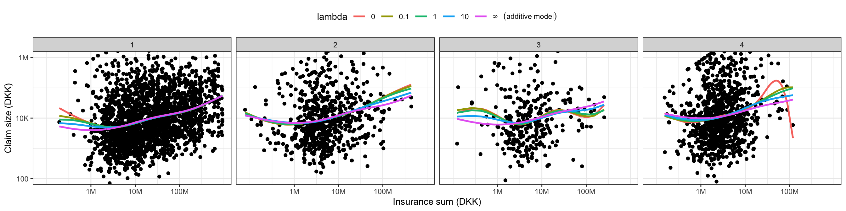
Figure 7.7 shows the resulting penalized model compared to the unpenalized interaction model (\(\lambda = 0\)) and the additive model (\(\lambda = \infty\)). A minimal penalization is enough to dampen the most pronounced spurious fluctuation for the fourth trade group considerably.
Code
tmp <- cbind(
    coefficients(claims_lm_spline_int),
    coef_hat,
    c(coefficients(claims_lm_spline_add), rep(0, 15))
)
pred <- cbind(claims[, c("sum", "grp")], exp(X %*% tmp))
pred <- tidyr::pivot_longer(pred, cols = !c(grp, sum), names_to = "lambda")
p0 + geom_line(
  aes(y = value, color = lambda),
  data = pred,
  linewidth = 1) +
  theme(legend.position = "top") +
  scale_color_discrete(
    expression(~lambda),
    labels = c(0, 0.1, 1, 10, expression(infinity~~~(additive~model)))
) 
In conclusion, we have found evidence in the data for an overall nonlinear relation between insurance sum and claim size plus an additive effect of trade group. For small insurance sums (less than DKK 1M) there is almost no relation, while for larger insurance sums there is roughly a linear relation on a log-log scale. The model fits the data well with a non-normal and slightly right skewed residual distribution, but as a predictive model it is weak, and insurance sum can together with trade group only explain 6–7% of the variation in the (log) claim size distribution.
To further investigate the computation of the penalized least squares estimates we present two alternatives to solving the normal equations. The penalized least squares estimates can, for instance, also be computed using the QR decomposition via the function lm.fit(). To achieve this we need to augment the model matrix and the outcome data suitably, as described in Section 2.5.2.
Another option diagonalizes \(\mathbf{X}^T \mathbf{X}\), which is beneficial if several penalized estimates for different choices of \(\lambda\) are to be computed. This is implemented in, e.g., the
lm.ridge() function in the package MASS, but only for \(\boldsymbol{\Omega} = \mathbf{I}\).Code
fit_lamb1 <- lm.fit(
    rbind(X, sqrt(0.1) * Omega),
    c(y, rep(0, ncol(Omega)))
)
fit_lamb2 <- lm.fit(
    rbind(X, sqrt(10) * Omega),
    c(y, rep(0, ncol(Omega)))
)
## Comparisons
range(coef_hat[, 1] - coefficients(fit_lamb1))
[1] -1.621947e-11 2.009581e-11Code
range(coef_hat[, 3] - coefficients(fit_lamb2)) [1] -2.994938e-12 6.206813e-12The results are again (numerically) identical to using solve() above.
A more general class of penalty functions are the elastic net penalties: \[ \mathrm{pen}_{\alpha}(\beta) = \frac{(1 - \alpha)}{2} \sum_{i=2}^p \gamma_i \beta_i^2 + \alpha \sum_{i=2}^p \gamma_i |\beta_i| \] where \(\alpha, \gamma_i \geq 0\) are tuning parameters that control the tradeoffs between different parameter coordinates and between the penalization of the square \(\beta_i^2\) vs. the absolute value \(|\beta_i|\).
The penalized least squared loss function \[
\beta \mapsto \frac{1}{2n} \| \mathbf{Y} - \mathbf{X} \beta\|^2 + \lambda \mathrm{pen}_{\alpha}(\beta)
\] is then minimized to find the parameter estimate \(\hat{\beta}^{\lambda, \alpha}\). This is implemented in the glmnet() function from the glmnet package. Setting \(\alpha = 0\), setting the \(\gamma_i\)-s to only penalize parameters affiliated with the interaction terms, and setting \(\lambda\) appropriately, we can (mostly) reproduce the results corresponding to \(\lambda = 1\) in the previous computations.
Note that the squared error loss is normalized by the sample size here. This is useful when penalizing to make the consequences of penalization with the same penalty function somewhat invariant to the sample size.
Code
claims_glmnet <-
  glmnet(
    X[, -1],
    y,
    lambda =  1 / length(y),
    alpha = 0,
    penalty.factor = c(rep(0, 8), rep(1, 15)),
    standardize = FALSE,
    control = list(thresh = 1e-20)
  )
The table below shows a comparison between the estimated parameters where the interaction model and the additive model are the two extremes, and where the different penalized models allow for interactions but dampen the parameter estimates.
Code
tmp <- cbind(
  coefficients(claims_lm_spline_int),
  coef(claims_glmnet),
  coef_hat,
  c(coefficients(claims_lm_spline_add), rep(0, 15))
) |> as.matrix()
model_names <- c("Int", "glmnet", "lamb=0.1", "lamb=1", "lamb=10", "Add")
colnames(tmp) <- model_names
tmp |> knitr::kable()| Int | glmnet | lamb=0.1 | lamb=1 | lamb=10 | Add | |
|---|---|---|---|---|---|---|
| (Intercept) | 10.7532578 | 9.0673669 | 9.5236459 | 9.0408248 | 8.8593137 | 8.8814820 |
| ns_log(sum)1 | -2.6251748 | -0.9568287 | -1.4299006 | -0.9227234 | -0.6347876 | -0.6003830 |
| ns_log(sum)2 | -1.4025686 | 0.2905587 | -0.1562128 | 0.3131589 | 0.4555315 | 0.4772376 |
| ns_log(sum)3 | -0.7423540 | 0.4849057 | 0.1262502 | 0.5141862 | 0.7964803 | 0.9362141 |
| ns_log(sum)4 | -1.5647812 | 1.6022533 | 0.7994661 | 1.6314972 | 1.6232581 | 1.1017271 |
| ns_log(sum)5 | 1.1076330 | 1.7740587 | 1.5584540 | 1.7969098 | 2.0847765 | 2.4040495 |
| grp2 | -1.1906322 | 0.5215829 | 0.1180383 | 0.5314214 | 0.5527723 | 0.5449651 |
| grp3 | -1.4599698 | 0.3803798 | 0.0922280 | 0.3790249 | 0.3991520 | 0.4237152 |
| grp4 | -0.5076130 | 0.7186348 | 0.2107849 | 0.7476949 | 0.8590757 | 0.9052219 |
| ns_log(sum)1:grp2 | 2.0112659 | 0.2794913 | 0.7448109 | 0.2485383 | -0.0516060 | 0.0000000 |
| ns_log(sum)2:grp2 | 1.4742819 | -0.2043732 | 0.1401766 | -0.1945614 | 0.0394280 | 0.0000000 |
| ns_log(sum)3:grp2 | 2.6491452 | 1.3435050 | 1.7496132 | 1.2955515 | 0.6004754 | 0.0000000 |
| ns_log(sum)4:grp2 | 2.9986180 | -0.4792694 | 0.3440967 | -0.4917850 | -0.2420562 | 0.0000000 |
| ns_log(sum)5:grp2 | 2.1464728 | 1.0053485 | 1.4734882 | 0.9410101 | 0.3300255 | 0.0000000 |
| ns_log(sum)1:grp3 | 1.0076599 | -0.5771570 | -0.4066957 | -0.5497631 | -0.2054750 | 0.0000000 |
| ns_log(sum)2:grp3 | 2.9934422 | 0.7908662 | 1.2773557 | 0.7483898 | 0.1737987 | 0.0000000 |
| ns_log(sum)3:grp3 | -0.9486629 | -1.4478141 | -1.6624656 | -1.3682998 | -0.4778804 | 0.0000000 |
| ns_log(sum)4:grp3 | 5.5282681 | 0.3394308 | 1.4633253 | 0.3035817 | 0.1602147 | 0.0000000 |
| ns_log(sum)5:grp3 | 2.9651748 | -0.0889754 | 0.8913097 | -0.1441994 | -0.1743938 | 0.0000000 |
| ns_log(sum)1:grp4 | 2.0440243 | 0.4184676 | 1.0059274 | 0.3683202 | 0.0288478 | 0.0000000 |
| ns_log(sum)2:grp4 | 0.7090661 | 0.4200314 | 0.7798192 | 0.4209364 | 0.5119487 | 0.0000000 |
| ns_log(sum)3:grp4 | 8.1703453 | 2.0003923 | 3.0525674 | 1.8590907 | 0.6269703 | 0.0000000 |
| ns_log(sum)4:grp4 | -42.4868426 | -0.8884066 | -2.1525621 | -0.8488293 | -0.5117852 | 0.0000000 |
| ns_log(sum)5:grp4 | -64.8214183 | 0.0992791 | -2.9952450 | 0.2050156 | 0.3326141 | 0.0000000 |
The glmnet() implements a fast and robust convex optimizer that works particularly well when computing estimates for a range of penalty parameters \(\lambda\) and/or \(\alpha\). It works across a range of standard generalized linear models and with the general class of penalty functions \(\mathrm{pen}_{\alpha}(\beta)\). It is therefore recommended for most practical applications of penalized regression with generalized linear models.
7.3.2 Nonlinear birth weight models
In Chapter 3 we found that the linear model of birth weight did not quite fit the data. As for the claim size models, we will use basis expansion to fix the lack of model fit.
We have to decide which relations to expand and how. We will use \(B\)-splines and thus we have to choose knot placement. We should be a little careful not to construct models tailor-made to capture nonlinear relations we have spotted by eye-balling residual plots, say. Since we then run the risk of overfitting to random fluctuations. In particular, formal downstream justifications using statistical tests are invalidated. The eye-balling process is a model selection procedure with statistical implications, which are difficult to account for.
Here we decided to expand gestationalAge using natural cubic splines with three knots in 38, 40, and 42 weeks. The boundary knots were determined by the range of the data set, and were thus 25 and 47. We also expanded age, but we let the ns() function determine the knots automatically for that predictor. The last continuous predictor, alcohol has a very skewed marginal distribution, and it was not judged to be suitable for a standard basis expansion. A formal test of the nonlinear effect is computed below as an \(F\)-test.
Code
form <- weight ~ gestationalAge +
                 age +
                 children +
                 coffee +
                 alcohol +
                 smoking +
                 abortions +
                 feverEpisodes

birth_weight_lm <- lm(form, data = birth_weight)
Nonlinear main effects model.
Code
nsg <- function(x)
    ns(x, knots = c(38, 40, 42), Boundary.knots = c(25, 47))

form <- weight ~ nsg(gestationalAge) +
    ns(age, df = 3) +
    children +
    coffee +
    alcohol +
    smoking +
    abortions +
    feverEpisodes

birth_weight_lm_spline <- lm(form, data = birth_weight)

anova(birth_weight_lm, birth_weight_lm_spline) |> knitr::kable()| Res.Df | RSS | Df | Sum of Sq | F | Pr(>F) |
|---|---|---|---|---|---|
| 11139 | 2537626346 | NA | NA | NA | NA |
| 11134 | 2466413420 | 5 | 71212926 | 64.29455 | 0 |
gestationalAge against the main effects model.
The main effects model is a submodel of the nonlinear main effects model. This is not obvious. The nonlinear expansion will result in 4 columns in the model matrix \(\mathbf{X}\), none of which being gestationalAge. However, the linear function is definitely a natural cubic spline, and it is thus in the span of the 4 basis functions. With \(\mathbf{X}'\) the model matrix for the main effects model, it follows that there is a \(\mathbf{C}\) such that Equation 2.12 holds. This justifies the use of the \(F\)-test. The conclusion from Table 7.4 is that the nonlinear model is highly significant.
Code
birth_weight_diag <- augment(birth_weight_lm_spline, data = birth_weight)
p1 <- ggplot(birth_weight_diag, aes(.fitted, .std.resid)) +
  stat_binhex(bins = 20) + binScale + geom_smooth(linewidth = 1, fill = "blue") +
  xlab("fitted values") + ylab("standardized residuals")
p2 <- ggplot(birth_weight_diag, aes(gestationalAge, .std.resid)) +
  stat_binhex(bins = 20) + binScale + geom_smooth(linewidth = 1, fill = "blue") +
  xlab("gestationalAge") + ylab("")
p3 <- ggplot(birth_weight_diag, aes(sample = .std.resid)) +
  geom_abline(intercept = 0, slope = 1, color = "blue", linewidth =  1) +
  geom_qq() +
  xlab("theoretical quantiles") + ylab("")
gridExtra::grid.arrange(p1, p2, p3, ncol = 3)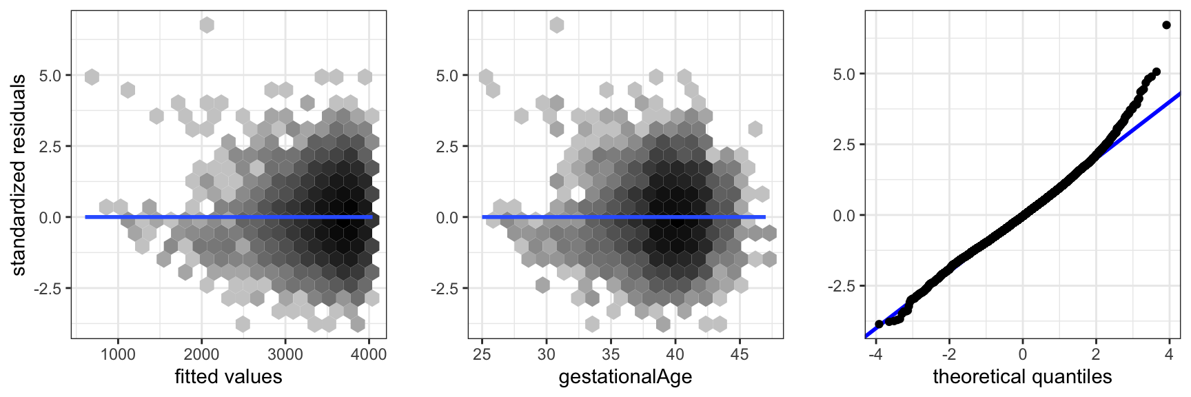
gestationalAge expanded using splines.
The positioning of the knots for spline expansion is selected based on the marginal distribution of the predictor7. The knots should be placed reasonably relative to the distribution of the predictor, so that we learn about nonlinearities where there is data to learn from. In this case we placed knots at the median and the 10% and 90% quantiles of the distribution of gestationalAge. The ns() function makes a similar automatic selection of knots based on the marginal distribution of the predictor variables when it is applied in the formula. One just has to specify the number of basis functions using the df argument.
7 Letting the knots be parameters to be estimated is not a statistically viable idea. The resulting estimation problem becomes computationally much more difficult, and it is not straightforward how to adjust subsequent statistical analyses to account for the data adaptive choice of knots.
An eye-ball decision based on Figure 3.8 would be that a single knot around 41 would have done the job, but we refrained from making such a decision. A subsequent test of the nonlinear effect with 1 degrees of freedom would not appropriately take into account how the placement of the knot was made.
Figure 7.8 shows diagnostic plots for the nonlinear main effects model. They show that the inclusion of the nonlinear effect removed the previously observed problem with assumption A1. The error distribution is still not normal, but right skewed with a fatter right tail than the normal distribution. There is a group of extreme residuals for preterm born children, which should be given more attention than they will be given here.
Reduced nonlinear main effects model.
Code
form <- weight ~ nsg(gestationalAge) +
    children +
    coffee +
    smoking

birth_weight_lm_spline_small <- lm(form, data = birth_weight)

anova(birth_weight_lm_spline_small, birth_weight_lm_spline) |>
knitr::kable()| Res.Df | RSS | Df | Sum of Sq | F | Pr(>F) |
|---|---|---|---|---|---|
| 11142 | 2469351552 | NA | NA | NA | NA |
| 11134 | 2466413420 | 8 | 2938131 | 1.657931 | 0.1032394 |
Table 7.5 shows that dropping the four weak predictors from the nonlinear main effects model is again borderline and not really significant.
Figure 7.9 shows examples of the fit for the reduced nonlinear main effects model. The figure illustrates the general nonlinear relation between weight and gestationalAge. Differences due to other variables are purely additive in this model, which amounts to translations up or down of the curve. The figure shows a couple of extreme cases; the majority group who have had children before and who do not smoke or drink coffee, and a minority group who have had children before and smoke and drink coffee the most. What we should notice is the wider confidence band on the latter (smoke = 3, coffee = 3) compared to the former, which is explained by the skewness of the predictor distributions. Table 7.6 gives confidence intervals for the remaining parameters based on the nonlinear main effects model.
Code
pred_frame <- expand.grid(
  children = factor(1),
  smoking = factor(c(1, 3)),
  coffee = factor(c(1, 3)),
  gestationalAge = seq(25, 47, 0.1),
  alcohol = 0,
  age = median(birth_weight$age),
  feverEpisodes = 0,
  abortions = factor(0)
)

pred <- predict(
  birth_weight_lm_spline,
  newdata = pred_frame,
  interval = "confidence"
)

pred_frame <- cbind(pred_frame, pred)

ggplot(pred_frame, aes(gestationalAge, fit, color = coffee)) +
  geom_line() + ylab("weight") +
  geom_ribbon(
    aes(ymin = lwr, ymax = upr, fill = coffee),
    alpha = 0.3
  ) + facet_grid(. ~ smoking, label = label_both)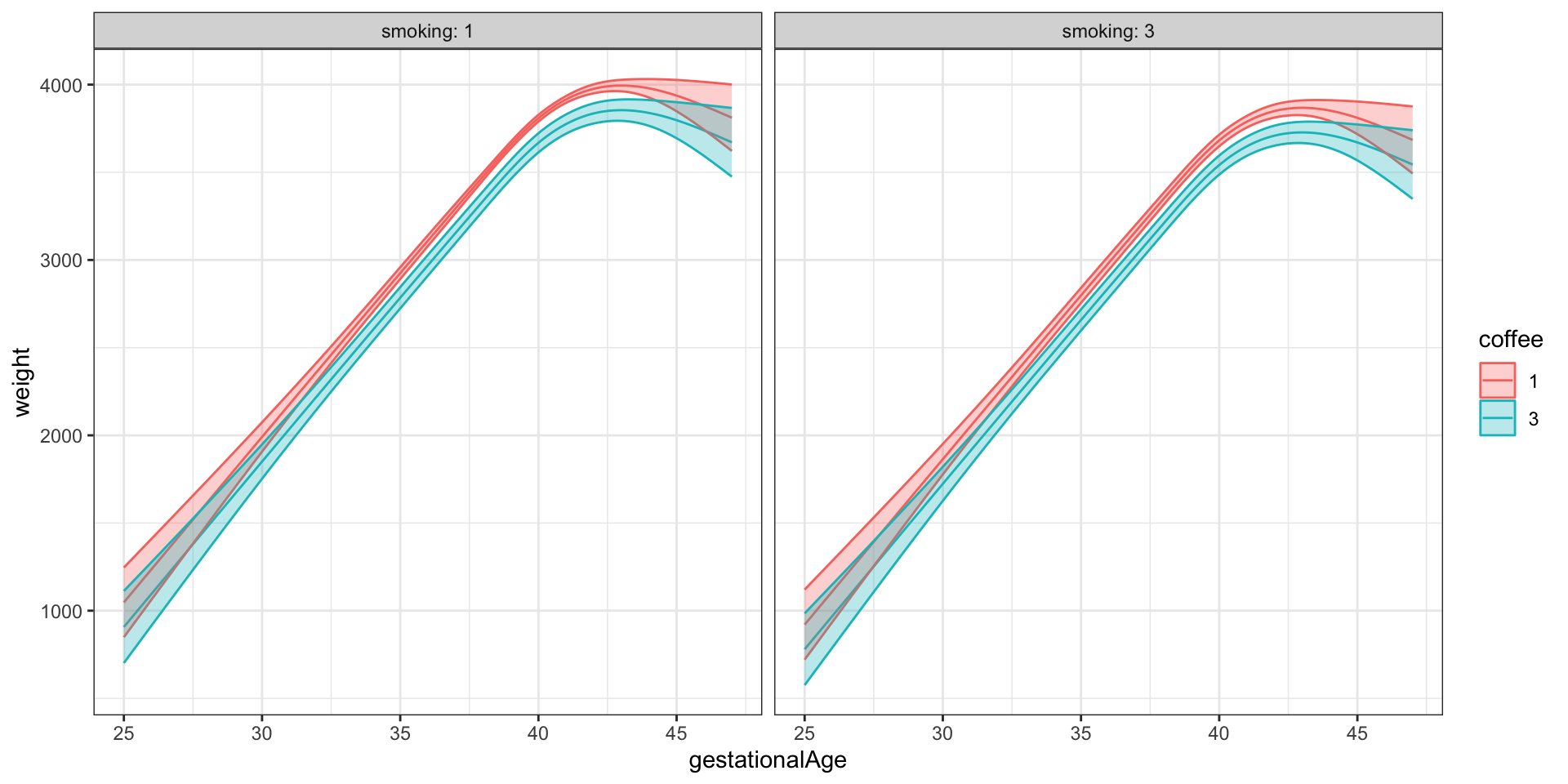
gestationalAge. Here illustrations of the fitted mean and 95% confidence bands for children=1.
| term | conf.low | conf.high |
|---|---|---|
| children1 | 155.470 | 194.087 |
| coffee2 | -82.608 | -42.431 |
| coffee3 | -193.020 | -87.630 |
| alcohol | -13.167 | 6.509 |
| smoking2 | -125.758 | -75.259 |
| smoking3 | -155.765 | -97.975 |
To conclude the analysis, we will again include interactions. However, the variable gestationalAge is in fact only taking the integer values 25 to 47, and the result of a nonlinear effect coupled with a third order interaction, say, results in an almost saturated model. That is, the interaction model has more or less a separate mean for all observed combinations of the predictors. We choose to consider a less complex model with all second order interactions between gestationalAge and the three factors that we have judged to be strong predictors.
Nonlinear interaction model.
Code
form <- weight ~ (smoking + coffee + children) * nsg(gestationalAge) +
   ns(age, df = 3) +
   alcohol +
   abortions +
   feverEpisodes

birth_weight_lm_spline_int <- lm(form, data = birth_weight)
Code
pred_frame <- expand.grid(
  children = factor(c(0, 1)),
  smoking = factor(c(1, 2, 3)),
  coffee = factor(c(1, 2, 3)),
  gestationalAge = 25:47,
  alcohol = 0,
  age = median(birth_weight$age),
  feverEpisodes = 0,
  abortions = factor(0)
)

pred <- predict(birth_weight_lm_spline_int, newdata = pred_frame, interval = "confidence")


pred_frame <- cbind(pred_frame, pred)
pred_frame$fit_spline <- predict(birth_weight_lm_spline, newdata = pred_frame)

ggplot(pred_frame, aes(gestationalAge, fit)) +
  geom_point(data = birth_weight, aes(y = weight), size = 0.3, alpha = 0.1) +
  facet_grid(coffee ~ children + smoking, label = label_both) +
  geom_ribbon(aes(ymin = lwr, ymax = upr), fill = gray(0.85)) +
  geom_line(color = "red") + coord_cartesian(ylim = c(0, 5000)) +
  geom_line(aes(y = fit_spline), color = "blue") + ylab("weight") +
  scale_y_continuous(breaks = c(1000, 2000, 3000, 4000))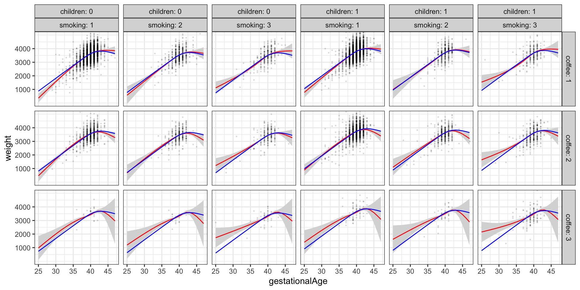
Figure 7.10 shows the predicted values for the reduced nonlinear main effects model for all combinations of children, smoking and coffee (blue curves). These curves are all just translations of each other. In addition, the figure shows the predicted values and a 95% confidence band as estimated with the nonlinear interaction model. We observe minor deviations for the reduced main effects model, which can explain the significance of the test, but the deviations appear unsystematic and mostly related to extreme values of gestationalAge. The conclusion is that even though the inclusion of interaction effects is significant, there is little to gain over the reduced nonlinear main effects model.
Code
anova(birth_weight_lm_spline, birth_weight_lm_spline_int) |>
knitr::kable(digits = 10)| Res.Df | RSS | Df | Sum of Sq | F | Pr(>F) |
|---|---|---|---|---|---|
| 11134 | 2466413420 | NA | NA | NA | NA |
| 11114 | 2451152208 | 20 | 15261213 | 3.459865 | 2.612e-07 |
Table 7.7 shows that inclusion of interaction terms is still significant by a formal statistical test. It is, however, always a good idea to visualize how the nonlinear interaction model differs from the model with only main effects as above instead of just focusing on the formal test. The test may, on the other hand, support the visualization as a quantification of whether the differences seen in a figure are actually statistically significant.
Exercises
Exercise 7.1 This is a continuation of Exercise 2.1.
Code
set.seed(04022016)
factor_labels <- rep(c("A", "B", "C"), each = 50)
formula_data <- tibble(
    x =  rnorm(150, 0),
    z = factor(sample(factor_labels)),
    mu = (z == "A") + cos(x) + 0.5 * (z == "B") * sin(x),
    y = rnorm(150, mu, 0.5)
)
Expansions can be achieved by applying an R function that returns a matrix of basis function evaluations when applied to a vector of predictor values. We consider a spline basis expansion.
Code
library(splines)
model.matrix(y ~ ns(x, df = 4), formula_data) |>
    head()
(Intercept) ns(x, df = 4)1 ns(x, df = 4)2 ns(x, df = 4)3 ns(x, df = 4)4
1 1 0.75361809 0.169569207 0.08775628 -0.04862859
2 1 0.07603605 -0.191091633 0.44504011 -0.25394848
3 1 0.77817043 0.005536704 0.13653515 -0.07790959
4 1 0.14168625 -0.207697339 0.48371373 -0.27601639
5 1 0.15040919 0.515081509 0.26234462 0.07216468
6 1 0.20011297 0.527404800 0.24317864 0.02930359Before you run the R expression below, answer the following question on the basis of what you have learned.
- Determine the number of columns for the model matrix below and explain and interpret what the columns mean?
Code
model.matrix(y ~ ns(x, df = 4) * z, formula_data) |>
    head()
Figure 7.11 was obtained by fitting the linear model using the model matrix, or rather the formula, from above. The figure illustrates the model fit by comparing the fitted model directly to the true means and via the residuals. Fitted values and residuals were computed using the augment() function from the broom package.
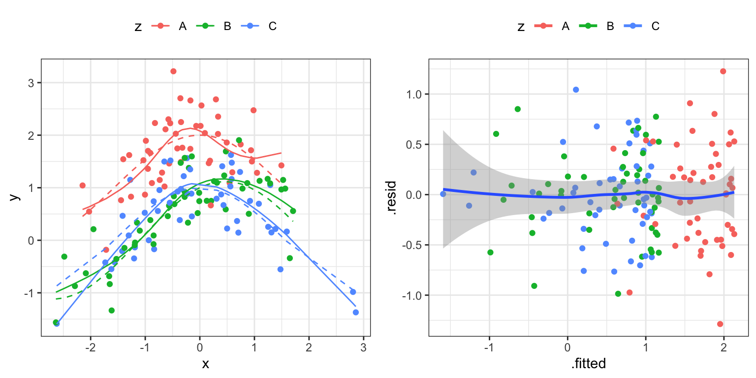
- Reproduce Figure 7.11 and discuss the model fit.
Exercise 7.2 Consider the following matrices
X <- splines::bs(
    seq(0, 1, 0.01),
    knots = c(0.3, 0.5, 0.7)
)
X_prime <- seq(0, 1, 0.01)
of \(B\)-spline basis functions evaluated on a grid in the interval \([0, 1]\). Use Exercise 2.3 to verify that X_prime is in the column space of X. You can use the formula from the exercise to compute \(\mathbf{C}.\) Can you also use lm.fit()?
Exercise 7.3 The regression function is called partially linear in the \(j\)-th variable if it is of the form \[ m(x) = \beta_j x_j + h_{-j}(x_{-j}). \]
- Find the partial dependence function for the \(j\)-th variable.
- Show that, just as for the linear model, \[ \beta_j = \frac{\mathrm{cov}(\varepsilon_{-j}, X_j)}{\mathbf{V}(X_j - r_j(X_{-j}))}. \]
- Discuss what kind of regression model you need of \(m_{-j}\) to be able to compute partial residuals.
Exercise 7.4 If the regression function has the form \[ m(x) = \beta_j(x_{-j}) x_j + h_{-j}(x_{-j}), \] it is affine in \(x_j\) for any fixed \(x_{-j}\). It is partially linear in the \(j\)-th variable but with a coefficient that depends on \(x_{-j}\).
- Compute the partial dependence function.
- Show that \[ \mathrm{cov}(\varepsilon_{-j}, X_j) = \mathbf{E}(\beta_j(X_{-j})v_j(X_{-j})), \] where \(v_j(X_{-j}) = \mathbf{V}(X_j - r_j(X_{-j}) \mid X_{-j})\) is a conditional variance.
Exercise 7.5 This exercise is based on the TitanicSurvival dataset from the carData package, which records the survival status, sex, age and passenger class of the 1309 passengers aboard the Titanic; see
?carData::TitanicSurvival
for details. If the carData package is not installed on your computer, you need to install it first.
Age is missing for around 20% of the passengers in the dataset, and these should be excluded for this analysis.
Code
data(TitanicSurvival, package = "carData")
titanic <- filter(TitanicSurvival, !is.na(age))
Figure 7.12 shows the empirical survival proportion within age bins, which suggests a nonlinear relation between age and the probability of survival.
Code
ggplot(titanic, aes(age, as.numeric(survived) - 1)) +
    stat_summary_bin(fun = mean, binwidth = 5, geom = "point") +
    ylab("Survival proportion")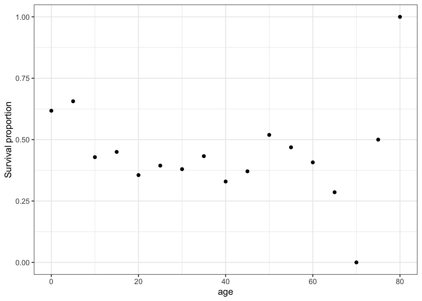
Fit an additive logistic regression model of
survivedonsex,ageandpassengerClass, treatingageas linear on the logit scale. Interpret the estimated coefficients.Assess whether the model fits the data by a residual plot (residuals against fitted values). Use
simulate()to simulate a few datasets from the fitted model, refit and compare their smoothed residual plots. Does the additive model seem adequate?Now fit an extended model by including second order interactions,
survived ~ sex*passengerClass*age.Assess if this model fits the data better.
Use
anova()to compute an “Analysis of Deviance Table” containing sequential deviance tests of a sequence of nested models. Explain the different models in the table and interpret the table.Extend the model further by expanding
ageusing natural cubic splines (ns(age, df = 3)) and refit the model. Visualize the fitted model by plotting the predicted survival probability againstage, separately for each combination ofsexandpassengerClass, together with pointwise confidence bands. Compare with the model from Question 3.