library(RwR)
library(ggplot2)
library(tibble)
library(dplyr)
library(tidyr)
library(skimr)
library(broom)
library(lubridate)
library(survival)
library(splines)11 Survival analysis
Warning
This chapter is still a draft and minor changes are made without notice. In particular, a few practical examples will be added in Sections 11.4 and 11.5.
This chapter deals with regression models for time-to-event data with possible right censoring, which is common for survival data but also in other applications of statistics1 such as reliability theory and credit risk.
1 Time to failure of an electronic component, say, or time default of a debitor.
Some of the notation in this chapter will deviate a bit from the notation used for other regression models, which is deliberate and to follow some of the standard conventions in the survival literature. The response variable will, for example, be denoted \(T\) instead of \(Y\), which is also a natural notation for a time-to-event observation. The regression models are, however, still of the form, where a linear predictor \(\eta = X^T \beta\) is formed from the vector of predictors \(X \in \mathbb{R}^p\) and a parameter \(\beta \in \mathbb{R}^p\), and the effect of the predictors on the survival distribution is then only through \(\eta\).
11.1 Outline and prerequisites
Section 11.2 is covers the basic definitions specific to survival analysis and motivates why survival (regression) analysis is special. It also covers the basic nonparametric estimators of survival distributions. Section 11.3 covers parametric survival models and likehood based methods for estimation and statistical inference. The accelerated failure time models and the proportional hazard model are introduced, which show two different ways that the linear predictor can affect the survival distribution. Section 11.4 primarily treats Cox’s proportional hazard model, which is the most widely used survival regression model. As the name suggests, it is a proportional hazard model, but the methodology is semiparametric, meaning in this case that a baseline hazard function is left unconstrained. Section 11.5 introduces survival residuals, which differ a bit from residuals considered for linear and generalized linear models. These differences reflect that survival models don’t target conditional expectations, but otherwise the purposes of the residuals for model diagnostics are the same.
The chapter primarily relies on the following R packages.
11.2 Introduction to survival analysis
A typical application of survival analysis is to the study of survival of patients after an initial diagnosis. In such a study, patients are enrolled whenever they are diagnosed with a given (serious, life threatening) disease. We refer to the time of enrollment2 as the baseline, and we note that the baseline for different patients can be different calendar times, and that the survival time is the time from baseline to death. The baseline is thus time zero on the time axis of the survival time.
2 For some applications, all individuals or units can have the same baseline, e.g., in an experiment on the longevity of electronic components, but in many applications the baseline calendar times differ among units. In credit risk models of time to default, say, the baseline could be the date of the loan application.
The patients are followed for some period of time, and if they die during this followup period, their survival time is registered. At a planned calendar time the study ends and the status of the patients are registered, that is, we register if they died, in which case we know their survival time, or if they are still alive. All patients alive at the end of the study have right censored survival times. This form of censoring is sometimes called administrative censoring. Some patients might also have dropped out of the study earlier, because they moved or didn’t want to participate anymore, say. At the time they drop out, we say that they are lost-to-followup, and this also results in right censoring of their survival time.
In addition to the, possibly right censored, survival times of the patients, we may collect additional data on the patients. We can then use some or all of such additional variables to construct a regression model of the survival distributions. But it is not clear that we want to model expected survival times, and the conditional expectation is often not3 the correct target of a survival regression model.
3 One reason is technical. Expectations rely on the tails of distributions, and with right censoring we don’t get that information.
Regression models for survival data thus differ from the linear and generalized linear regression models in at least the following two ways:
- There is almost always a censoring mechanism, and certain aspects of the data are consequently missing. We need to deal with this in the modeling.
- Survival distributions are skewed distributions on the positive half line. It is often the shape of the distribution rather than the location of the distribution that is of interest.
The overall objective of a survival regression model is the same as for any regression model: how are the different predictors associated with the survival time. We might then have different more specific questions we want to answer. For example, to determine if the survival distributions depends on a choice of treatment (testing). Or we might want to quantify how strongly a predictor is associated with survival response.
We might, of course, also be interested in prediction, which we often call survival prognosis. It is rarely of interest to make a point prediction of a survival time for an individual, but we might report a prediction interval (the interquartile range, say), or we might report probabilistic predictions in terms of an entire (conditional) survival distribution.
Example 11.1 We will throughout this chapter use a dataset on prostate cancer survival, which is included in the RwR package as the dataset prostate. The data is from a randomized clinical trial on prostate cancer patients with four different treatments (one placebo and three different dosages of estrogen). There are 502 patients in the trial, and we will in this chapter focus on four of the variables.
rx: Treatment encoded as a factor.status: Either the cause of death or indication that the patient was alive at the end of study.dtime: The censored survival time since baseline in months.age: The baseline age of the patient in years.
There are several other variables included in the dataset, and among these are sdate: the date that the patient entered the study. We will not use sdate for modeling, but it is used in Figure 11.1 to visualize the data. For later purposes, the data is converted to a tibble.
Code
data(prostate, package = "RwR") # version >= 0.3.5
prostate <- prostate |> as_tibble()
# A tibble: 502 × 5
rx status dtime age sdate
<fct> <fct> <dbl> <dbl> <date>
1 0.2 mg estrogen alive 72 75 1977-08-10
2 0.2 mg estrogen dead - other ca 1 54 1977-09-21
3 5.0 mg estrogen dead - cerebrovascular 40 69 1978-01-12
4 0.2 mg estrogen dead - cerebrovascular 20 75 1978-03-19
5 placebo alive 65 67 1978-03-22
6 0.2 mg estrogen dead - prostatic ca 24 71 1978-06-14
7 placebo dead - heart or vascular 46 75 1978-06-27
8 placebo alive 62 73 1978-06-28
9 1.0 mg estrogen alive 61 60 1978-08-01
10 1.0 mg estrogen alive 60 78 1978-08-07
# ℹ 492 more rows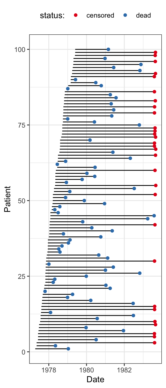
Figure 11.1 illustrates the data for the first 100 patients that enter the study. The figure shows their entry date (baseline), their survival time from that date and the status indicator when follow-up ends, indicating if they are dead or if the survival time is censored.
Since the treatments were randomly assigned, differences in the survival distributions between the four treatment groups can be ascribed to the treatment alone. That is, the treatments can be interpreted as the causes of any such differences. We will first of all be interested in testing if there are effects of treatment as well as estimating the magnitudes of such effects.
There are other variables included in the dataset, such as age, and we could use these variables for two different purposes. We could use the variables for prognostic purposes, that is, for fitting regression models that give more accurate survival prognoses for individual patients. Another purpose could be to investigate heterogeneity of treatment effects, that is, to investigate if the treatment works differently on different subgroups of the patients.
11.2.1 Survival distributions and censoring
A survival time \(T^*\) is simply a non-negative random variable. We will denote its distribution function by \(F\), and if the distribution has density \(f\) w.r.t. Lebesgue measure, we have \[ F(t) = P(T^* \leq t) = \int_{0}^{t} f(s) \mathrm{d}s. \] The corresponding survival function of \(T^*\) is \[ S(t) \coloneqq 1 - F(t) = P(T^* > t) = \int_t^{\infty} f(s) \mathrm{d} s. \]
In terms of \(S\) we define the cumulative hazard function as \[ \Lambda(t) \coloneqq - \log(S(t)), \tag{11.1}\] so that \[ S(t) = \exp\left(-\Lambda(t)\right). \tag{11.2}\] If \(S\) is continuously differentiable, \(-S'(t) = f(t)\) is the density of the survival distribution, and the hazard function is defined as \[ \lambda(t) \coloneqq - (\log S(t))' = \frac{f(t)}{S(t)}. \tag{11.3}\]
There are one-to-one relations between the distribution function, the survival function and the cumulative hazard function.
We can observe that \[ \begin{align*} \lambda(t) & = \lim_{\varepsilon \to 0+} \frac{1}{\varepsilon} \frac{F(t+\varepsilon) - F(t)}{S(t)} \\ & = \lim_{\varepsilon \to 0+} \frac{1}{\varepsilon} P(T^* \in (t,t+\varepsilon] \, | \, T^* > t), \end{align*} \] and \(\lambda(t)\) thus has the interpretation as the instantaneous rate of death at time \(t\) given survival beyond time \(t\). We also note that \[ \Lambda(t) = \int_0^t \lambda(s) \mathrm{d} s = - \log S(t) \] which explains why \(\Lambda\) is called the cumulative hazard function.
We will not observe \(T^*\) but only \[ T = \min\{T^*, C\} \quad \text{ and } \quad \delta = 1(T^* \leq C) \] for a censoring variable \(C\). We call \(T\) the right censored survival time and \(\delta\) the status indicator. The status indicator is \(1\) if the \(T\) is uncensored and \(0\) otherwise. To distinguish the distribution of \(C\) clearly from the distribution of the survival time, we will generally denote its survival function by \(H\) and its density by \(h\) (if it exists). That is, \[ H(t) = P(C > t) = \int_t^\infty h(s) \mathrm{d} s. \]
11.2.2 Model assumptions
We will generally consider \(n\) observations and let \(T^*_1, \ldots, T^*_n\) denote the survival times and \(C_1,\ldots,C_n\) the censoring times. We then observe the right censored survival times \[ T_i = \min\{T_i^*, C_i\} \] and the status indicators \[ \delta_i = 1(T_i^* \leq C_i) \] for \(i = 1, \ldots, n\).
The vector of predictor variables is as elsewhere denoted \(X_i \in \mathbb{R}^p\), and we are generally interested in models of the conditional distributions4 \[ T_i^* \mid X_i = x. \]
4 Note that the target is the conditional distribution of the unobserved and uncensored \(T^*_i\), not the oberved and censored \(T_i\).
An issue of particular concern for survival analysis is when a predictor variable is observed. In some studies, some potential predictor variables are monitored throughout the study. Such variables as BMI and blood pressure might be recorded on a monthly basis, say. It is possible to develop a general time-to-event theory where predictors also change with time, but it is both technically beyond this chapter, and it is also conceptually challenging to understand and interpret such models correctly.
We will throughout assume that all predictors are observed5 at or before baseline, and we refer to such predictors as baseline predictors.
5 Or, as a minimum, observable at time zero.
The modeling assumptions across the different individuals are now straightforward modifications of A5 or A6 to the survival setup.
SA5: The conditional distribution of \((T^*_i, C_i)\) given \(\mathbf{X}\) depends only on \(X_i\) and \((T^*_1, C_1), \ldots, (T^*_n, C_n)\) are conditionally independent given \(\mathbf{X}\).
SA6: The triples \((T^*_1, C_1, X_1), \ldots, (T^*_n, C_n, X_n)\) are i.i.d.
Since \((T_i, \delta_i)\) is a function of \((T^*_i, C_i)\), then either assumption implies the same distributional statement about the \((T_i, \delta_i)\)-s as about the \((T^*_i, C_i)\)-s.
An additional delicate survival modeling question is what to assume about the joint distribution of \(T^*_i\) and \(C_i\) (possibly, conditionally on \(X_i\)). Throughout, we will make the following assumption.
Independent censoring: \(T^*_i\) and \(C_i\) are conditionally independent given \(X_i\).
Even though the assumption above is a conditional independence statement, it is known simply as “independent censoring”. In the literature, “independent censoring” may refer to a slightly more permissive assumption (Definition III.2.1 in Andersen et al. (1993)), stating that information about censoring status at any given timepoint is not allowed to affect the residual survival distribution beyond that timepoint. For this chapter we will make the stronger, but simpler, independent censoring assumption as stated above.
Andersen, Per Kragh, Ørnulf Borgan, Richard D. Gill, and Niels Keiding. 1993. Statistical Models Based on Counting Processes. Springer Series in Statistics. New York: Springer-Verlag.
11.2.3 The Kaplan-Meier and Nelson-Aalen estimators
If \(T_1^*, \ldots, T_n^*\) are i.i.d. and if they were observed, we could define the empirical survival function \[ \hat{S}^*_n(t) = \frac{1}{n} \sum_{i=1}^n 1(T_i^* > t) \] as a nonparametric estimator of \(S\). Clearly, we cannot compute \(\hat{S}^*_n\) if we only have censored observations. The purpose of this section is to introduce two nonparametric estimators of a survival distribution when the survival times are i.i.d. and independently censored6.
6 In this section there are no predictors, and we effectively assume that \((T_1^*, C_1), \ldots, (T_n^*, C_n)\) are i.i.d. and that \(T_i^*\) and \(C_i\) are independent.
To handle the censoring we introduce the individuals at risk at time \(t\): \[ Y(t) = \sum_{i=1}^n 1(t \leq T_i). \] It can be computed based on the censored survival times, and it counts how many individuals have survived to time \(t\) and are uncensored at that time.
Definition 11.1 below gives the general definition of the Kaplan-Meier estimator of the survival function, but to motivate this definition, we first suppose that there are no ties among the observed survival times, that is, where we have strict inequalities among the ordered survival times \[ T_{(1)} < T_{(2)} < \ldots < T_{(n-1)} < T_{(n)}. \] Here \(T_{(k)}\) denotes the survival time with rank \(k\), and we will denote the corresponding status indicator by \(\delta_{(i)}\).
Without censoring, the Kaplan-Meier estimator equals \(\hat{S}^*\), cf. Exercise 11.2
When there are no ties, and \(T_{(k)} \leq t < T_{(k+1)}\), we can factorize the survival function as \[ \begin{align*} S(t) & = P(T^* > t) \\ & = P(T^* > t \mid T^* \geq T_{(k)}) \times P(T^* \geq T_{(k)} \mid T^* \geq T_{(k-1)}) \\ & \hspace{5mm} \ldots \times P(T^* \geq T_{(2)} \mid T^* \geq T_{(1)}) \times P(T^* \geq T_{(1)}) \\ \end{align*} \] where \(P(T^* \geq T_{(i+1)} \mid T^* \geq T_{(i)})\) is the conditional probability of surviving from \(T_{(i)}\) to \(T_{(i+1)}\) given survival beyond time \(T_{(i)}\).
Since \(Y(T_{(i)})\) are the number of individuals at risk7 at time \(T_{(i)}\) and \(Y(T_{(i)}) - \delta_{(i)}\) are the number of individuals that die in the interval \([T_{(i)}, T_{(i+1)})\), we can regard \[ \frac{Y(T_{(i)}) - \delta_{(i)}}{Y(T_{(i)})} = 1-\frac{\delta_{(i)}}{Y(T_{(i)})} \] as an estimator of the conditional probability \(P(T^* \geq T_{(i+1)} \mid T^* \geq T_{(i)})\). This gives the Kaplan-Meier estimator for \(t \in [T_{(k)}, T_{(k+1)})\) \[ \hat{S}(t) = \left(1-\frac{\delta_{(k)}}{Y(T_{(k)})}\right) \cdots \left(1-\frac{\delta_{(2)}}{Y(T_{(2)})}\right) \left(1-\frac{\delta_{(1)}}{Y(T_{(1)})}\right). \]
7 Alive and uncensored.
We can write the Kaplan-Meier estimator in a slightly more abstract notation as \[ \hat{S}(t) = \prod_{i: T_i \leq t} \left(1-\frac{\delta_i}{Y(T_i)}\right). \tag{11.4}\]
To define the Kaplan-Meier estimator that allows for multiple deaths at the same time (ties), we introduce the counting process of deaths (non-censored events) \[N(t) = \sum_{i=1}^n 1(T_i \leq t, \delta_i=1),\] and the jumps for the counting process given as \[\Delta N(t) = N(t) - N(t-) = N(t) - \lim_{\epsilon \to 0+} N(t-\epsilon),\]
Definition 11.1 With the above notation, the Kaplan-Meier estimator is defined as \[ \hat{S}(t) = \prod_{s \leq t} \left(1-\frac{\Delta N(s)}{Y(s)}\right). \tag{11.5}\]
In the infinite product above, all factors where \(\Delta N(s) = 0\) are equal to \(1\). There is thus only a finite number of factors different from \(1\). When \(\Delta N(s) \in \{0, 1\}\) we see that Equation 11.5 coincides with Equation 11.4. The definition allows for \(\Delta N(s) > 1\) to correctly account for multiple deaths at the same time and thus ties among the observed survival times.
The function
survfit() from the R package survival can be used to compute the Kaplan-Meier estimator.Since the cumulative hazard function is \(\Lambda = - \log(S)\), we can estimate it nonparametrically as \[ - \log(\hat{S}(t)) = - \sum_{s \leq t} \log \left(1-\frac{\Delta N(s)}{Y(s)}\right). \tag{11.6}\] But there is also a different, and direct, nonparametric estimator of the cumulative hazard function. The logic behind this estimator is that for a differentiable survival function \(S\) and \(t > s\) (but \(t - s\) small),
\[ \begin{align*} P(T^* \in [s, t) \mid T^* \geq s) & = \frac{S(s) - S(t)}{S(s)} \\ & \approx - \frac{S'(s)}{S(s)}(t - s) = \lambda(s)(t - s). \end{align*} \]
By a Riemann sum approximation we see that \[ \Lambda(t) \approx \sum_{i: T_{(i)} \leq t} P(T^* \in [T_{(i)}, T_{(i + 1)}) \mid T^* \geq T_{(i)}), \] and if there are no ties, the conditional probabilities in the sum above can be estimated8 as \(\delta_{(i)} / Y(T_{(i)})\). This leads to the Nelson-Aalen estimator \[ \hat{\Lambda}(t) = \sum_{i: T_{(i)} \leq t} \frac{\delta_{(i)}}{Y(T_{(i)})}. \tag{11.7}\]
8 Either \(\delta_{(i)} = 1\) and one individual out of \(Y(T_{(i)})\) dies in the interval (at time \(T_{(i)}\)), or \(\delta_{(i)} = 0\) and no individuals die in the interval.
The general definition below allows for multiple deaths at the same time.
Definition 11.2 The Nelson-Aalen estimator of the cumulative hazard function is
\[
\hat{\Lambda}(t) = \sum_{s \leq t} \frac{\Delta N(s)}{Y(s)}.
\tag{11.8}\]
Since the survival function is given by \(S(t) = \exp(-\Lambda(t))\), we can estimate the survival function by plugging the Nelson-Aalen estimator of the cumulative hazard, which gives \[ \exp\left(-\hat{\Lambda}(t)\right) = \prod_{s \leq t} \exp\left(- \frac{\Delta N(s)}{Y(s)}\right). \tag{11.9}\]
We note that \(\exp(-\hat{\Lambda})\) is not the Kaplan-Meier estimator and nor is \(- \log(\hat{S})\) the Nelson-Aalen estimator.
The function
survfit() with argument stype = 2 estimates the survival function in terms of the Nelson-Aalen estimator via Equation 11.9.The mismatch between the Kaplan-Meier and the Nelson-Aalen estimators is a small nuisance, but we may note that \[ \exp\left(- \frac{\Delta N(s)}{Y(s)}\right) \approx \left(1 - \frac{\Delta N(s)}{Y(s)}\right) \] for large \(Y(s)\) by using the Taylor expansion \(\exp(x) = 1 + x + o(x^2)\). Thus differences between the factors are small unless \(s\) is so large that the number of individuals at risk, \(Y(s)\), is small.
One can argue that the way ties are handled above presumes that survival times can be exactly equal, which is at odds with any continuous survival distribution. If we regard ties as a consequence of lack of precision in our registration or due to rounding of the survival times, it makes sense to replace \(\frac{\Delta N(s)}{Y(s)}\) by \[ \frac{1}{Y(s)} + \frac{1}{Y(s) - 1} + \ldots + \frac{1}{Y(s) - \Delta N(s) + 1}. \] This is known as the Fleming-Harrington correction for ties. It often doesn’t make much of a practical difference tough.
The function
survfit() with argument ctype = 2 will use the Fleming-Harrington correction for ties.Example 11.2 We continue Example 11.1 by first considering a summary of the marginal distributions of the four variables.
Code
select(prostate, c(rx, status, dtime, age)) |> skim()Variable type: factor
| skim_variable | n_missing | complete_rate | ordered | n_unique | top_counts |
|---|---|---|---|---|---|
| rx | 0 | 1 | FALSE | 4 | pla: 127, 1.0: 126, 5.0: 125, 0.2: 124 |
| status | 0 | 1 | FALSE | 10 | ali: 148, dea: 130, dea: 96, dea: 31 |
Variable type: numeric
| skim_variable | n_missing | complete_rate | mean | sd | p0 | p25 | p50 | p75 | p100 | hist |
|---|---|---|---|---|---|---|---|---|---|---|
| dtime | 0 | 1 | 36.13 | 23.32 | 0 | 14.25 | 34 | 57.75 | 76 | ▇▆▅▆▆ |
| age | 1 | 1 | 71.46 | 7.08 | 48 | 70.00 | 73 | 76.00 | 89 | ▁▂▅▇▁ |
prostate dataset.
Table 11.1 shows 148 patients (out of 502) were alive at the end of the study. Thus 148 of the survival times are right censored. Table 11.2 shows a more detailed tabulation of the values of the status variable, which specifies one out of nine different causes of death – in addition to specifying if the patient is still alive. We may also note that the survival time (dtime) is registered in months since baseline, which is a very coarse scale. Consequently there are many ties in the data.
| status | Freq |
|---|---|
| alive | 148 |
| dead - cerebrovascular | 31 |
| dead - heart or vascular | 96 |
| dead - other ca | 25 |
| dead - other specific non-ca | 28 |
| dead - prostatic ca | 130 |
| dead - pulmonary embolus | 14 |
| dead - respiratory disease | 16 |
| dead - unknown cause | 7 |
| dead - unspecified non-ca | 7 |
We will fit a survival distribution, using either of the nonparametric estimators above, where we ignore the information about different causes of death. Thus the status variable will only be used to determine the censoring status.
We fit survival functions for all patients using the survfit() function from the survival package. See ?survfit.formula for details about how to specify a model using the formula interface. Note that the left hand side of the formula, that specifies the response, uses the special Surv() function syntax to include information about the censoring status. We fit the survival functions below using both the Kaplan-Meier and the Nelson-Aalen, and we also fit the survival function using the Nelson-Aalen estimator with the Fleming-Harrington correction for ties.
Code
prostate_KM <- survfit(
    Surv(dtime, status != "alive") ~ 1,
    data = prostate,
)

prostate_NA <- survfit(
    Surv(dtime, status != "alive") ~ 1,
    data = prostate,
    stype = 2
)

prostate_NA_FH <- survfit(
    Surv(dtime, status != "alive") ~ 1,
    data = prostate,
    stype = 2,
    ctype = 2
)
Figure 11.2 shows the fitted survival curves – including a plot that zooms in on a part of the curves. The differences are small and barely visible, and they are most pronounced in the tail of the distribution.
Code
p1 <- summary(prostate_KM, data.frame = TRUE) |>
        ggplot(aes(time, surv)) +
        geom_step(data = summary(prostate_NA, data.frame = TRUE), color = "blue") +
        geom_step(data = summary(prostate_NA_FH, data.frame = TRUE), color = "red") +
        geom_step() +
        ylim(0, 1) +
        xlab("time (months)") +
        ylab("survival probability")

p2 <- p1 + coord_cartesian(xlim = c(50, 75), ylim = c(0.20, 0.40))

gridExtra::grid.arrange(p1, p2, ncol = 2)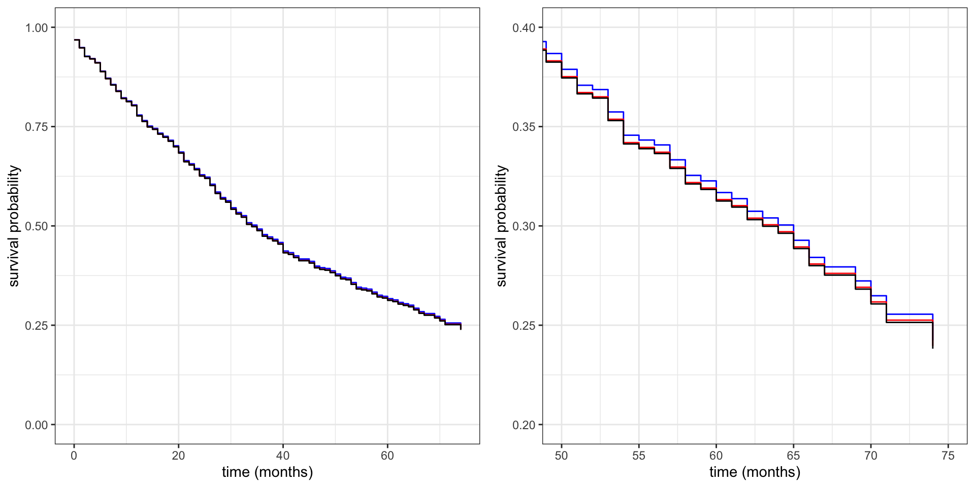
We then fit a separate survival function for each treatment group. We can think about this as a simple regression model with a single categorical predictor variable (the treatment variable rx), and the formula specification below is similar to other regression model specifications. The main difference is that using survfit() we fit a survival function for each treatment group instead of a mean value, say.
Code
prostate_KM_rx <- survfit(
    Surv(dtime, status != "alive") ~ rx,
    data = prostate
)
Code
summary(prostate_KM_rx, data.frame = TRUE) |>
        ggplot(aes(time, surv, color = strata)) +
        geom_step() +
        ylim(0, 1) +
        xlab("time (months)") +
        ylab("survival probability") +
        theme(legend.position = "top")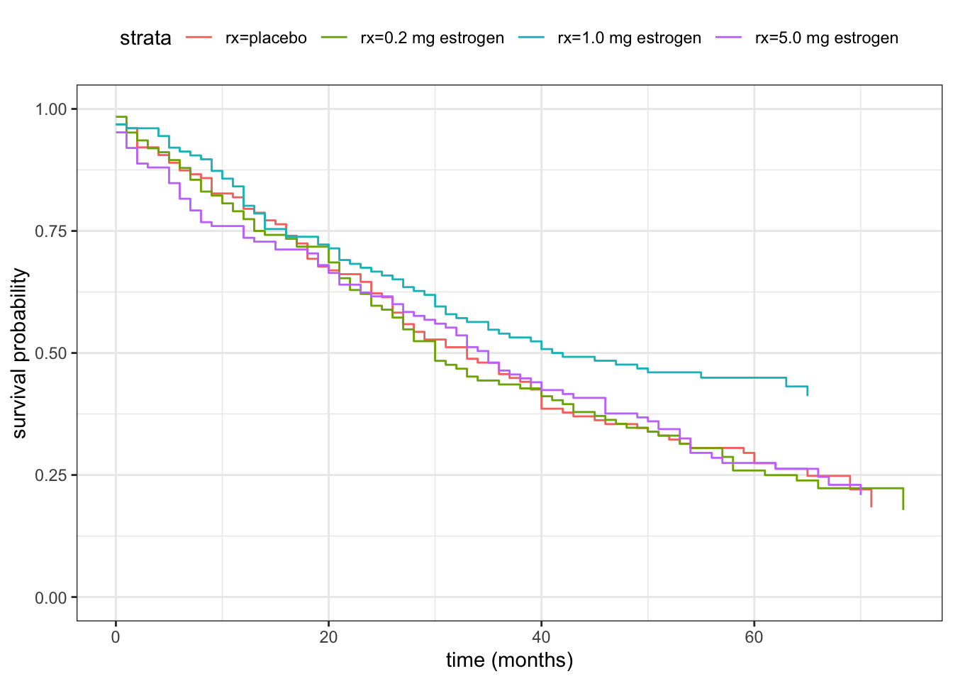
11.3 Parametric survival models
In this section we focus on parametric models of the survival distribution, and we will first derive a generic expression for the likelihood function. We then turn to regression models and introduce the accelerated failure time models and the proportional hazards models as two different was for the predictors to affect the response distribution.
11.3.1 The likelihood
Recall that in terms of \(T^*\) and \(C\) we have \(T = \min\{T^*, C\}\) and \(\delta = 1(T^* \leq C)\). Our first result gives the density of the joint distribution of \((T, \delta)\) in terms of the marginal distributions of \(T^*\) and \(C\) when they are independent.
Theorem 11.1 If \(T^*\) and \(C\) are independent the joint distribution of \((T, \delta)\) has density \[ g(t, \delta) = f(t)^\delta S(t)^{1-\delta} h(t)^{1-\delta} H(t)^\delta \] w.r.t. the product measure \(m \otimes \tau\) (Lebesgue measure times the counting measure).
Proof. First note that \[ \begin{align*} P(T \leq t, \delta = 1) & = P(T^* \leq t, \delta = 1) \\ & = P(T^* \leq t,C \geq T^*) \\ & = \int_0^t f(s) \int_s^{\infty} h(u) \mathrm{d} u \mathrm{d} s \\ & = \int_0^t f(s) H(s) \mathrm{d} s. \end{align*} \] Likewise, \[ P(T \leq t, \delta = 0) = \int_0^t h(s) S(s) \mathrm{d} s, \] and we conclude that the density is \[ g(t, \delta) = \left\{ \begin{array}{ll} f(t) H(t) & \text{if } \delta = 1 \\ h(t) S(t) & \text{if } \delta = 0. \end{array} \right. \]
Based on the density result above we can introduce the full likelihood for right censored observations. With \((T_1, \delta_1), \ldots, (T_n, \delta_n)\) independent the full likelihood is \[ L = \prod_{i=1}^n f_i(T_i)^{\delta_i} S_i(T_i)^{1-{\delta_i}} h_i(T_i)^{1-{\delta_i}} H_i(T_i)^{\delta_i}. \]
For a parametrized model of the distributions of \(T^*_1, \ldots, T^*_n\) we have that \(f_i = f_{i, \beta}\) for some parameter \(\beta\). The censoring distributions, given by the densities \(g_i\), usually hold no information about the parameter \(\beta\). This implies that \[ L(\beta) = \prod_{i=1}^n f_{i, \beta}(T_i)^{\delta_i} S_{i, \beta}(T_i)^{1-{\delta_i}} K_i \] with \(K_i\) depending on the observations but not the parameter \(\beta\).
Note how the derivation of the likelihood makes it explicit what the dominating measure is, and thus that the joint distribution in fact has a density. The derivation also makes it clear how the distribution of the censoring mechanism enters, and why it can be ignored when it does not depend on the unknown parameter \(\beta\). The argument for ignorance is not independent censoring9 but that the \(g_i\)-s do not depend upon \(\beta\). Technically, the censoring distribution and the parameter \(\beta\) are variation independent.
9 Though independent censoring does play a role here for our particular derivation and form of the full likelihood.
By dropping the factors \(K_i\), that do not depend upon the parameter \(\beta\), in the expression above for the likelihood, we arrive at the following definition of the survival likelihood.
Definition 11.3 With the above setup, the survival likelihood is \[ L(\beta) = \prod_{i=1}^n f_{i, \beta}(T_i)^{\delta_i} S_{i, \beta}(T_i)^{1-{\delta_i}}. \tag{11.10}\]
It is possible to take a slightly different point of view and condition on the censoring variables instead. Then the dominating measure for the \(i\)-th censored observation, \(T_i\), becomes \(m + \delta_{C_i}\) (\(\delta_{C_i}\) is the Dirac measure in \(C_i\)). One arrives at the same likelihood as above though.
We can also express the likelihood in terms of the hazard and cumulative hazard functions.
Proposition 11.1 If \(f_{i, \beta}\) has hazard function \(\lambda_{i,\beta}\) and cumulative hazard function \(\Lambda_{i, \beta}\), the survival likelihood equals \[ L(\beta) = \prod_{i=1}^n \lambda_{i, \beta}(T_i)^{\delta_i} e^{- \Lambda_{i, \beta}(T_i)} \tag{11.11}\]
Proof. Recall that \[ \lambda_{i, \beta}(t) = \frac{f_{i,\beta}(t)}{S_{i,\beta}(t)} \] and that \[ S_{i,\beta}(t) = e^{- \Lambda_{i, \beta}(t)}. \] Hence \[ \begin{align*} L(\beta) & = \prod_{i=1}^n f_{i, \beta}(T_i)^{\delta_i} S_{i, \beta}(T_i)^{1-{\delta_i}} \\ & = \prod_{i=1}^n \lambda_{i, \beta}(T_i)^{\delta_i} S_{i, \beta}(T_i)^{\delta_i} S_{i, \beta}(T_i)^{1-{\delta_i}} \\ & = \prod_{i=1}^n \lambda_{i, \beta}(T_i)^{\delta_i} S_{i, \beta}(T_i) \\ & = \prod_{i=1}^n \lambda_{i, \beta}(T_i)^{\delta_i} e^{- \Lambda_{i, \beta}(T_i)}. \end{align*} \]
Example 11.3 The Weibull distribution has hazard function \[ \lambda(t) = \alpha \gamma t^{\gamma - 1} \] for \(\alpha, \gamma > 0\) two parameters. The special case \(\gamma = 1\) gives us the exponential distribution with constant hazard function. The Weibull distribution has increasing hazard functions over time when \(\gamma > 1\) and decreasing hazard function when \(\gamma < 1\).
The cumulative hazard function is \[ \Lambda(t) = \alpha \int_0^t \gamma s^{\gamma - 1} \mathrm{d} s = \alpha t^\gamma. \]
For right censored i.i.d. observations from the Weibull model, the likelihood becomes \[ L(\alpha, \gamma) = \prod_{i=1}^n (\alpha \gamma)^{\delta_i} T_i^{\delta_i(\gamma - 1)} e^{- \alpha T_i^\gamma}, \] and the log-likelihood is \[ \begin{align*} \ell(\alpha, \gamma) & = \log L(\alpha, \gamma) \\ & = \sum_{i=1}^n \delta_i (\log(\alpha) + \log(\gamma) + (\gamma - 1)\log(T_i)) - \alpha T_i^\gamma. \end{align*} \]
Example 11.4 (MLE for the exponential distribution) Continuing Example 11.3 and fixing \(\gamma = 1\), corresponding to an exponential distribution with hazard rate \(\alpha\), we find that the log-likelihood equals \[ \ell(\alpha) = \sum_{i=1}^n \delta_i \log(\alpha) - \alpha T_i \] up to additive terms that do not depend on \(\alpha\). This log-likelihood has a unique stationary point \[ \hat{\alpha} = \frac{\sum_{i=1}^n \delta_i}{\sum_{i=1}^n T_i} = \frac{n_u}{\sum_{i=1}^n T_i} \] where \(n_u = \sum_{i=1}^n \delta_i\) are the number of deaths (the number of uncensored events). The second derivative of of \(\ell\) is negative, so \(\ell\) is concave and \(\hat{\alpha}\) is the MLE.
If we had treated the observations as if there were no censoring, we would get the MLE \[ \frac{n}{\sum_{i=1}^n T_i} > \hat{\alpha}, \] which overestimates the rate.
If we, on the other hand, discard the censored observations, we would get the MLE \[ \frac{n_u}{\sum_{i=1}^n \delta_i T_i} > \hat{\alpha}, \] which likewise overestimates the rate.
11.3.2 Regression models
We introduce two ways that predictor variables can affect the survival response distribution. The accelerated failure time models exemplified by the log-logistic model, and the proportional hazards models exemplified by the Weibull model. In the latter case, it turns out that the likelihood can be computed and optimized using methods for Poisson generalized linear models.
Accelerated failure time models
Example 11.5 (Log-logistic distribution) Suppose \(Z\) has a logistic distribution with distribution function \[ G(z) = \frac{e^{\lambda z}}{1 + e^{\lambda z}}. \] The distribution of \(T^* = e^Z\) is then the log-logistic distribution, whose distribution function is \[ F(t) = G(\log(t)) = \frac{t^{\lambda}}{1 + t^{\lambda}}, \] with corresponding density \[ f(t) = F'(t) = \frac{\lambda t^{\lambda-1}}{(1+t^{\lambda})^2} \] for \(t > 0\).
Definition 11.4 Let \(G\) be a distribution function (on \(\mathbb{R}\)). The corresponding accelerated failure time (AFT) model has survival function given as \[ S_{\eta} (t) = 1 - G( (\log(t) - \eta)/\sigma) \] with \(\eta = X^T \beta\) the linear predictor and \(\sigma > 0\) a scale parameter.
The AFT model is a scale-location model of the log-survival time.
The interpretation of the AFT model is that a unit change of the \(j\)-th predictor increases – or accelerates – the failure time by a factor \(e^{\beta_j}\).
Example 11.6 (Log-logistic AFT model) If \(G\) is the logistic distribution with scale parameter is \(\sigma = \lambda^{-1}\), the survival function for the corresponding AFT model is \[ \begin{align*} S_{\eta}(t) & = \frac{1}{1 + e^{\lambda(\log(t) - \eta)}} \\ & = \frac{1}{1 + e^{-\lambda \eta} t^{\lambda}}. \end{align*} \tag{11.12}\] where \(\eta = X^T \beta\) is the linear predictor. This is a log-logistic distribution as introduced in Example 11.5. The effect of \(\eta\) is10 a scale transformation of the log-logistic distribution with scale parameter \(e^{\eta}\). The density is \[ \begin{align*} f_{\eta}(t) & = \frac{\lambda e^{-\lambda \eta} t^{\lambda-1}}{(1+e^{-\lambda \eta} t^{\lambda})^2} \\ & = \frac{\lambda e^{\lambda (\log(t) - \eta)} t^{-1}}{(1+e^{\lambda(\log(t) - \eta)})^2}. \end{align*} \tag{11.13}\]
10 If \(T\) has log-logistic distribution with density \(f_0\), then \(e^{\eta} T\) is log-logistic distributed with density \(f_{\eta}\), cf. Exercise 11.1.
For maximum likelihood estimation we need to compute and optimize the likelihood in Equation 11.10. Efficient computation requires access to the density as well as the survival function, which are both explicitly available for the log-logistic distribution, which makes this distribution attractive for AFT models.
Example 11.7 We implement the negative log-likelihood (nll()) for the AFT model with a log-logistic survival distribution below. The implementation is based on Equation 11.10 using the expressions (11.12) and (11.13) for the survival function and density, respectively, of the log-logistic distribution.
The nll() function takes four arguments. Besides a vector of parameters (par), the censored survival times (time) and the status indicator (status), it takes a single additional argument x representing a categorical variable with \(k\) values. The parameter vector par is of the form \[
(\sigma, \beta_0, \ldots, \beta_{k-1}) = (\lambda^{-1}, \beta_0, \ldots, \beta_{k-1})
\] with \(\sigma\) the scale parameter, \(\beta_0\) the intercept and \(\beta_1, \ldots, \beta_{k-1}\) are contrasts. The survival function is also implemented below for later usage.
Code
# Argument `x` is an integer representing the k levels of a single
# categorical predictor variable. `par[2:(k+1)]` are the k
# beta-parameters corresponding to the intercept and contrasts.
# Its default value corresponds to no predictor.
nll <- function(par, time, status, x = rep(1, length(time))) {
    lambda <- par[1]^{-1}
    eta <- par[2] + c(0, par[-c(1, 2)])[x] # beta_x
    uncens <- status == 1
    lt <- log(time)
    logf <- (log(lambda) - lambda * eta[uncens] + (lambda - 1) * lt[uncens] -
        2 * log(1 + exp(lambda * (lt[uncens] - eta[uncens])))) |> sum()
    logS <- log(1 + exp(lambda * (lt[!uncens] - eta[!uncens]))) |> sum()
    - logf + logS
}
We use optim() with method L-BFGS-B to compute the maximum-likelihood estimate of a single survival distribution. Since some of the patients have survived less than one months, some survival times are registered as \(0\), which is first of all numerically problematic (due to \(\log(0)\)). For this reason we offset all times by \(0.5\) corresponding to shifting all death times by half a months.
Code
prostate_aft <- optim(
    c(2, 2),
    nll,
    method = "L-BFGS-B",
    lower = c(0.01, -Inf),
    time = prostate$dtime + 0.5, # to avoid log(0)
    status = prostate$status != "alive"
)
prostate_aft[1:2]
$par
[1] 0.8219375 3.5378103
$value
[1] 1758.922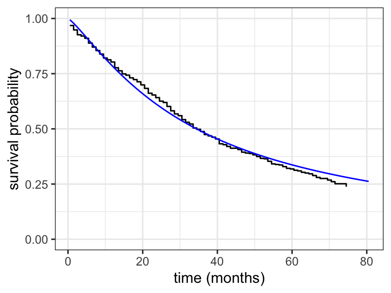
We see from the optim() result that the parameter estimates are \(\hat{\sigma} =\) 0.82 and \(\hat{\beta}_0 =\) 3.54, and we can also see that \(-\ell(\hat{\sigma}, \hat{\beta}_0) =\) 1758.92 The corresponding fitted survival function is compared to the Kaplan-Meier estimator in Figure 11.4.
We can also use our implementation to fit the regression model where the survival distribution depends on treatment.
Code
prostate_aft_rx <- optim(
    c(2, 2, 0, 0, 0),
    nll,
    method = "L-BFGS-B",
    lower = c(0.1, -Inf, -Inf, -Inf, -Inf),
    time = prostate$dtime + 0.5, # to avoid log(0)
    status = prostate$status != "alive",
    x = as.numeric(prostate$rx)
)
prostate_aft_rx[1:2]
$par
[1] 0.81992315 3.48305068 -0.04002854 0.33958359 -0.05824063
$value
[1] 1755.851Code
# The log-logistic survival function in the scale-location parametrization.
time0 <- 0:80
fit <- tibble(
    time = rep(time0, 4),
    surv = c(
        S(time0 + 0.5, prostate_aft_rx$par[1], prostate_aft_rx$par[2]),
        S(time0 + 0.5, prostate_aft_rx$par[1], prostate_aft_rx$par[2] + prostate_aft_rx$par[3]),
        S(time0 + 0.5, prostate_aft_rx$par[1], prostate_aft_rx$par[2] + prostate_aft_rx$par[4]),
        S(time0 + 0.5, prostate_aft_rx$par[1], prostate_aft_rx$par[2] + prostate_aft_rx$par[5])
    ),
    strata = rep(paste("rx=", levels(prostate$rx), sep = ""), each = 81)
)

summary(prostate_KM_rx, data.frame = TRUE) |>
        ggplot(aes(time + 0.5, surv, color = strata)) +
        geom_step(linetype = 2) +
        geom_line(data = fit) +
        ylim(0, 1) +
        xlab("time (months)") +
        ylab("survival probability") +
        theme(legend.position = "top")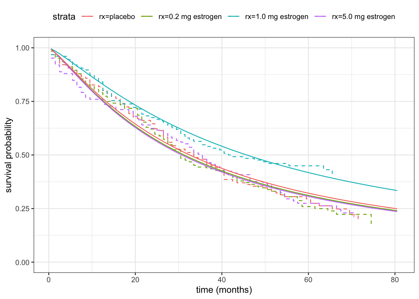
We can fit AFT models, and a range of other parametric regression models, via the survreg() function from the survival package.
Code
survreg(
    Surv(dtime + 0.5, status != "alive") ~ rx,
    data = prostate,
    dist = "loglogistic"
)
Call:
survreg(formula = Surv(dtime + 0.5, status != "alive") ~ rx,
data = prostate, dist = "loglogistic")
Coefficients:
(Intercept) rx0.2 mg estrogen rx1.0 mg estrogen rx5.0 mg estrogen
3.48297715 -0.03983952 0.33947524 -0.05802741
Scale= 0.8199158
Loglik(model)= -1755.9 Loglik(intercept only)= -1758.9
Chisq= 6.14 on 3 degrees of freedom, p= 0.105
n= 502 Note that the parametrization used by survreg() is exactly the same as we implemented, and that the estimated parameter values and computed log-likelihood are the same as well (up to small numerical differences).
The survreg() function even gives a likelihood-ratio test statistic (Chisq) of the hypothesis that there are no differences between the treatments. The corresponding \(p\)-value is computed using an approximating \(\chi^2\)-distribution with \(3\) degrees of freedom. It is above \(0.1\) and we cannot reject that there is no treatment effect.
As for lm and glm objects there are methods for survreg objects implemented in the broom package fo the glance() and tidy() functions and in the survival package for anova(). We will illustrate some of their usages in subsequent examples.
Proportional hazards models
A different model class is given by letting the linear predictor have a multiplicative effect on the hazard function. The resulting proportional hazards models are among the most widely used survival models.
Definition 11.5 With \(\lambda_0\) a baseline hazard function, the proportional hazards model is given by the hazard function \[ \lambda(t) = \lambda_0(t) e^{\eta} \] with \(\eta\) the linear predictor.
It follows that for the cumulative hazard function, \[ \Lambda(t) = \Lambda_0(t) e^{\eta}, \] and the proportionality holds for the cumulative hazard as well. The factor \(e^{\beta_j}\) is the hazard ratio between two models corresponding to a unit change of the \(j\)-th predictor.
The proportional hazards model is sometimes called the Cox model. Cox (1972) discovered that for the proportional hazards model, the parameters that enter into the linear predictor can be estimated without specifying the baseline hazard function. This will be covered in Section 11.4. Here we will instead show how the parameters can be estimated via maximum-likelihood when the baseline is assumed to be a Weibull distribution.
Cox, D. R. 1972. “Regression Models and Life-Tables.” Journal of the Royal Statistical Society. Series B (Methodological) 34 (2): pp. 187–220.
Example 11.8 The Weibull baseline hazard function and cumulative hazard function are
\[
\lambda_0(t) = \gamma t^{\gamma-1} \quad \text{and} \quad \Lambda_0(t) = t^{\gamma}.
\] The log-likelihood is \[
\begin{align*}
\ell & = \sum_{i=1}^n \delta_i \log(\gamma T_i^{\gamma-1}e^{\eta_i}) - T_i^{\gamma}e^{\eta_i} \\
& = \underbrace{\sum_{i=1}^n \delta_i \log(T_i^{\gamma}e^{\eta_i}) - T_i^{\gamma}e^{\eta_i}}_{\text{Poisson log-likelihood}} +
\sum_{i=1}^n \delta_i \log(\gamma T_i^{-1}).
\end{align*}
\] This is (surprisingly) up to a constant the log-likelihood for a Poisson model of the \(\delta_i\)-s with logarithmic link function and mean value \(T_i^{\gamma}e^{\eta_i}\) for fixed \(\gamma\). Note that the \(\alpha\) parameter appearing in Example 11.3 is captured by an intercept in the linear predictor.
For a fixed value of the linear predictor we also find that \[ \partial_{\gamma} \ell = \sum_{i=1}^n (\delta_i- T_i^{\gamma} e^{\eta_i}) \log T_i + \frac{\delta_i}{\gamma}. \] Thus \(\gamma\) solves the equation \[ \gamma = \frac{n_u}{\sum_{i=1}^n (T_i^{\gamma} e^{\eta_i} -\delta_i)\log T_i} \tag{11.14}\] with \(n_u\) the number of uncensored observations.
A practical algorithm can alternate between: i) estimate the linear predictor as \(\hat{\eta}^{(k)}\) by optimizing the Poisson log-likelihood (for fixed \(\gamma^{(k-1)}\)); and ii) update \[
\gamma^{(k)} = \frac{n_u}{\sum_{i=1}^n (T_i^{\gamma^{(k-1)}} e^{\hat{\eta}_i^{(k)}} -\delta_i)\log T_i}.
\]
The example above shows how implementations of generalized linear models – and Poisson regression models, in particular – can be used to fit the Weibull proportional hazards model (for fixed \(\gamma\)) with the survival times entering as an offset term. This was of historical importance as it made computations practical early on using some standard algorithms available. Today, the connection between the survival likelihood for Weibull distributions and the Poisson likelihood is mostly of theoretical and historical interest.
To fit the model we will instead show that the proportional hazards model with a Weibull baseline hazard function is also an accelerated failure time model, which makes it possible to use survreg() to fit the model.
Example 11.9 If we take \(G\) in Definition 11.4 to be the extreme value distribution \[ G(z) = 1 - \exp(-e^{z}), \] then the corresponding AFT model has survival function \[ S_\eta(t) = \exp\left(-(e^{-\eta}t)^{\frac{1}{\sigma}}\right) = \exp\left(-e^{-\gamma \eta}t^\gamma\right) \] where \(\gamma = \frac{1}{\sigma}\). That is, the cumulative hazard function is , which is the proportional hazards model with a Weibull baseline, but reparametrized in terms of the scale parameter \(\sigma = \frac{1}{\gamma}\), and the linear predictor is multiplied by \(-\gamma\).
We can use the survreg() function to fit the model.
Code
prostate_survreg <- survreg(
    Surv(dtime + 0.5, status != "alive") ~ rx,
    data = prostate,
    dist = "weibull"
)
prostate_survreg |> tidy()
# A tibble: 5 × 5
term estimate std.error statistic p.value
<chr> <dbl> <dbl> <dbl> <dbl>
1 (Intercept) 3.87 0.105 36.9 1.05e-297
2 rx0.2 mg estrogen -0.0314 0.148 -0.212 8.32e- 1
3 rx1.0 mg estrogen 0.392 0.161 2.43 1.49e- 2
4 rx5.0 mg estrogen -0.00534 0.149 -0.0358 9.71e- 1
5 Log(scale) 0.0222 0.0470 0.472 6.37e- 1We can compute the estimated survival functions for the Weibull model much in the same way as we did above for the log-logistic model, where we used the MLE of the parameters and the explicit formula for the survival function. However, this is a bit cumbersome and does not generalize well. We can instead use the predict() method for survreg objects to predict quantiles for the survival functions, which implicitly also gives the estimated survival functions.
Code
fit <- tibble(rx = factor(1:4, labels = levels(prostate$rx)))
p_seq <- seq(0.01, 0.90, 0.01)
pred <- predict(prostate_survreg, newdata = fit, type = "quantile", p = p_seq)
fit <- cbind(fit, as_tibble(pred, .name_repair = "minimal")) |>
    pivot_longer(cols = !rx, values_to = "time") |>
    mutate(
        surv = 1 - rep(p_seq, 4),
        strata = paste("rx=", rx, sep = "")
    ) |>
    filter(time <= 80)

summary(prostate_KM_rx, data.frame = TRUE) |>
        ggplot(aes(time + 0.5, surv, color = strata)) +
        geom_step(linetype = 2) +
        geom_line(data = fit, aes(time)) +
        ylim(0, 1) +
        xlab("time (months)") +
        ylab("survival probability") +
        theme(legend.position = "top") +
        xlim(0, 82)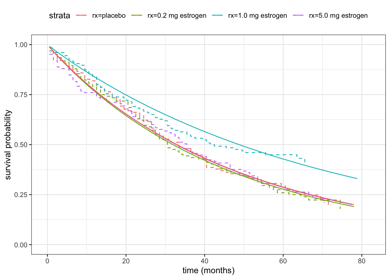
Figure 11.6 compares the fitted Weibull distributions to the Kaplan-Meier estimators for the four treatment groups, and Table 11.4 reports the test statistic and \(p\)-value for testing if there are no differences between the four treatment groups. The \(p\)-value is a bit smaller in this case than when using the log-logistic distribution, and this time just below 5%.
Code
prostate_survreg |>
    anova() |>
    select(-4) |>
    tidy() |>
    filter(term == "rx") |>
knitr::kable(digits = 3)| term | df | deviance | df.residual | p.value |
|---|---|---|---|---|
| rx | 3 | 9.619 | 497 | 0.022 |
To corroborate the technical relation between the log-linear Poisson regression model and the proportional hazards model with a Weibull baseline, we refit the \(\beta\)-parameters using glm() (fixing the scale parameter at its estimated value).
Code
sigma <- prostate_survreg$scale
glm((status != "alive") ~ offset(log(dtime + 0.5) / sigma) + rx,
    data = prostate,
    family = "poisson"
) |> coefficients() * (- sigma)
(Intercept) rx0.2 mg estrogen rx1.0 mg estrogen rx5.0 mg estrogen
3.870053562 -0.031447138 0.392042914 -0.005335812 glm() and identical to those in Table 11.3.
To conclude our analyses of the prostate survival times, we have shown how one treatment group (1.0 mg estrogen) has a slightly different survival distribution than the other three with a better survival prognosis. The statistical tests of any treatment effect, based on two parametric models, are at best borderline significant though, and we cannot draw any clear conclusion.
There do not seem to be any detectable difference between the other three treatment groups. It is particularly noteworthy that the treatment group with the highest dose (5.0 mg estrogen) have a survival distribution simular to the placebo group. If there were an effect, we would often expect it to be monotone in dosage, and it would be peculiar if the effect is only there for the medium dose.
11.4 Semiparametric survival models
For the parametric proportional hazards models in Definition 11.5, the baseline hazard function \(\lambda_0\) is either known or parametrized itself. There is a risk that we have misspecified this baseline model, and we would like to avoid a model of the baseline hazard if possible. This leads to the semiparametric proportional hazards model, where an individual’s hazard is proportional to a common baseline hazard \(\lambda_0\) with an individual weight factor, but where we do not model11 the baseline \(\lambda_0\).
11 This is similar to not making distributional assumptions such as A3 or GA3 for the linear and generalized models.
12 The \(i\)-th weight could be \(e^{\eta_i}\) with \[\eta_i = X_i^T \beta\] the linear predictor, but it does not need to be for the general arguments.
The general proportional hazards model assumes that the dependence of the predictors is via a multiplicative factor on the baseline, and the \(i\)-th individual thus has hazard function \[ \lambda_i(t) = w_i \lambda_0(t) \] for \(w_i > 0\) a weight12. The cumulative hazard function is consequently \(\Lambda_i(t) = w_i \Lambda_0(t)\).
Definition 11.6 In terms of the observations \(T_1, \ldots, T_n\) and weights \(w_1, \ldots, w_n \geq 0\) we define the cumulative weight process \[ W(t) = \sum_{j: t \leq T_j} w_j \] and the cumulative weights \(W_i = W(T_i)\).
Proposition 11.2 When \(\Lambda_i(t) = w_i \Lambda_0(t)\) the likelihood equals \[ L = \prod_{i: \delta_i = 1} \frac{w_i}{W_i} \left(\prod_{i} (W_i \lambda_0(T_i))^{\delta_i}\right) e^{-\int_0^{\infty} W(t) \lambda_0(t) \mathrm{d} t}. \]
To ease notation we leave out limits on the generic index \(i\) in products and sums. It will always run through observations from \(1\) to \(n\).
Proof. First note that with \(W(t) = \sum_{j: t \leq T_j} w_j\), \[
\sum_{i} \Lambda_i(T_i) = \int_0^{\infty} W(t) \lambda_0(t) \mathrm{d} t.
\] The likelihood can therefore be factorized as
\[
\begin{align*}
L & = \prod_{i} \lambda_i(T_i)^{\delta_i} e^{-\Lambda_i(T_i)} \\
& = \left(\prod_{i: \delta_i = 1} (w_i \lambda_0(T_i))^{\delta_i}\right) e^{-\int_0^{\infty} W(t) \lambda_0(t)
\mathrm{d} t} \\
& = \prod_{i: \delta_i = 1} \frac{w_i}{W_i} \left(\prod_{i}
(W_i \lambda_0(T_i))^{\delta_i}\right) e^{-\int_0^{\infty} W(t) \lambda_0(t)
\mathrm{d} t}.
\end{align*}
\]
The purpose of Proposition 11.2 is to decompose the likelihood into two factors, where the second factor \[ \tilde{L}(\lambda_0) = \left(\prod_{i} (W_i \lambda_0(T_i))^{\delta_i}\right) e^{-\int_0^{\infty} W(t) \lambda_0(t) \mathrm{d} t}. \] is the only one depending on \(\lambda_0\). This factor can be made arbitrarily large if we try to maximize over \(\lambda_0\), and there is thus no unconstrained “maximum-likelihood” estimator of \(\lambda_0\) in a classical sense.
It is possible to formalize, via a certain renormalization, that for fixed weights the “maximizer” is a generalized function of the form \[ \hat{\lambda}_0 = \sum_{i} \frac{\delta_i}{W_i} \delta_{T_i} \] where \(\delta_{T_i}\) is the Dirac measure in \(T_i\). Since \[ \int_0^{\infty} W(t) \hat{\lambda}_0 \mathrm{d} t = \sum_{i} W_i \frac{\delta_i}{W_i} = \sum_{i} \delta_i = n_u, \] the number of uncensored obervations, this leads to \[ \tilde{L}(\hat{\lambda}_0) = e^{-n_u}, \] which is independent of the weights. We pursue a similar perspective in Section 11.4.2.
11.4.1 Cox’s partial likelihood
Proposition 11.2 and the subsequent discussion suggest that for estimation of the parameters that enter into the weights13, and not into \(\lambda_0\), we can ignore the factor \(\tilde{L}\) in the likelihood. This motivates our definition of Cox’s partial likelihood.
13 And are variation independent with \(\lambda_0\).
Definition 11.7 Cox’s partial likelihood for the proportional hazards model is \[ L_{\mathrm{par}} = \prod_{i: \delta_i = 1} \frac{w_i}{W_i} \] where the cumulative weights \(W_i\) are given by Definition 11.6.
In practice, the predictors are mostly linked to the weights via an exponential function and are thus of the form \[
w_i = e^{X^T_i \beta} = e^{\eta_i}.
\tag{11.15}\] In this case we find that the partial log-likelihood equals
\[
\ell_{\mathrm{par}}(\beta) =
\sum_{i: \delta_i = 1} X_i^T \beta - \log \Bigg(\underbrace{\sum_{j: T_i \leq T_j} w_j}_{W_i} \Bigg),
\tag{11.16}\] with corresponding score function \[
\mathcal{U}_{\mathrm{par}}(\beta) = D \ell_{\mathrm{par}}(\beta) = \sum_{i: \delta_i = 1} X_i^T -
\frac{\sum_{j: T_i \leq T_j} X_j^T w_j}{W_i}
\tag{11.17}\] and information function
\[ \begin{align*} \hskip -30mm \mathcal{J}_{\mathrm{par}}(\beta) & = - D^2 \ell_{\mathrm{par}}(\beta) \\ & = \sum_{i: \delta_i = 1} \frac{\sum_{j: T_i \leq T_j} X_j X_j^T w_j}{W_i} - \frac{(\sum_{j: T_i \leq T_j} X_j w_j) (\sum_{j: T_i \leq T_j} X_j w_j)^T}{W_i^2}. \end{align*} \tag{11.18}\]
The estimate, \(\hat{\beta}\), is computed by maximizing \(\ell_{\mathrm{par}}\), and the observed information, \(\mathcal{J}(\hat{\beta}),\) is used for quadratic approximations of \(\ell_{\mathrm{par}}\), for standard error estimates and Wald tests. In practice, the computations proceed just as if \(\ell_{\mathrm{par}}\) were a log-likelihood function.
The particular score test \[ \mathcal{U}(0)^T \mathcal{J}(0)^{-1} \mathcal{U}(0) \] for testing \(\beta = 0\) reduces to a classical test known as the log-rank test in the special case with only a single categorical predictor.
Example 11.10 Cox’s proportional hazards model can be fitted to data via the function coxph() from the survival R package.
Code
prostate_cox <- coxph(
    Surv(dtime + 0.5, status != "alive") ~ rx,
    data = prostate,
)
prostate_cox |> tidy()
# A tibble: 3 × 5
term estimate std.error statistic p.value
<chr> <dbl> <dbl> <dbl> <dbl>
1 rx0.2 mg estrogen 0.0321 0.145 0.221 0.825
2 rx1.0 mg estrogen -0.386 0.157 -2.46 0.0140
3 rx5.0 mg estrogen 0.00291 0.146 0.0200 0.984 Code
anova(prostate_cox) |>
    tidy() |>
    filter(term == "rx") |>
knitr::kable(digits = 3)| term | logLik | statistic | df | p.value |
|---|---|---|---|---|
| rx | -2005.899 | 9.709 | 3 | 0.021 |
The parameter estimates are comparable to those obtained by survreg() with the Weibull distribution, by appropriately rescaling, since that model is parametrized as an AFT model. In particular, they Cox model regression parameters have the opposite sign. This is noteworthy, since a negative value of a Cox model regression parameter means that the corresponding predictor has a positive association with the survival time. That is, if \(\beta_i < 0\) then a unit increase of \(X_i\) decreases the hazard by a factor \(e^{-\beta_i} < 1\), which results in a survival distribution with longer survival times.
Note that the (partial) likelihood-ratio test reported in Table 11.7 results in a very similar conclusion as using the Weibull baseline.
11.4.2 Poisson empirical likelihood
To provide an additional perspective on Cox’s partial likelihood, we will show how it can also be derived from a rigorous profiling argument of the Poisson empirical likelihood we define below. Our main purpose of giving this argument is that we then also get an explicit formula for a nonparametric estimator of the cumulative baseline hazard function.
For \(\lambda_1, \ldots, \lambda_n \geq 0\) we define the corresponding jump cumulative hazard function as \[ \Lambda(t) = \sum_{i : T_i \leq t} \lambda_i. \] We can regard this cumulative hazard function as having the hazard function \[ \lambda(t) = \sum_{i} \lambda_i \delta_{T_i}, \] which is, of course, not a function but a measure, and \(\Lambda(t)\) is the measure of the interval \([0, t]\). The measure has point mass \(\lambda_i\) in the jump point \(T_i\).
Definition 11.8 The Poisson empirical likelihood of a jump cumulative hazard function is \[ L^*(\Lambda) = \prod_{i} \lambda_i^{\delta_i} e^{- \Lambda_i} \] where \(\Lambda_i = \Lambda(T_i)\).
In this section we think about \(L^*\) as simply a formal extension of the likelihood (11.11) from continuously differentiable cumulative hazard functions to jump functions, but see also Section 11.6 on discrete time survival distributions, and see Johansen (1983) for a justification of \(L^*\) as a real likehood.
Johansen, Søren. 1983. “An Extension of Cox’s Regression Model.” International Statistical Review 51 (2): 165–74.
The next lemma gives an expression for the Poisson empirical log-likelihood for jump cumulative hazard functions of the form \[ \Lambda_i(t) = w_i \sum_{j: T_j \leq t} e^{h_j}. \]
Lemma 11.1 Suppose that \(\Lambda_0\) has jumps \(\lambda_i = e^{h_i}\) for \(h_i \in \mathbb{R}\). For the proportional hazards model with baseline \(\Lambda_0\) the Poisson empirical log-likelihood is \[ \ell^* = \sum_{i} \delta_i h_i + \delta_i \log (w_i) - e^{h_i} W_i. \tag{11.19}\]
Proof. The Poisson log-likelihood for the proportional hazards model is \[ \begin{align*} \ell^* & = \sum_{i} \delta_i \log(\lambda_0(T_i)) + \delta_i \log (w_i) - \Lambda_0(T_i)w_i \\ & = \sum_{i} \delta_i h_i + \delta_i \log(w_i) - w_i \sum_{j : T_j \leq T_i} e^{h_j}, \end{align*} \] where \(\ell^*\) is expressed in terms of the weights and the exponents \(h_j\). Interchanging the sums in the log-likelihood we get \[ \ell^* = \sum_{i} \delta_i h_i + \delta_i \log (w_i) - e^{h_i} W_i. \]
Lemma 11.2 The maximizer of \(\ell^*\) in (11.19) over \(h_1, \ldots, h_n\) is given by \[ e^{h_i} = \frac{\delta_i}{W_i} \] for \(i = 1, \ldots, n\).
With all weights being \(1\) in Lemma 11.2, the estimator is recognized as the Nelson-Aalen estimator.
Proof. The parameters \(h_i\) are variation independent, and we can thus maximize the function by maximizing each term. Differentiating we find that \[ \partial_{h_i} \ell^* = \delta_i - e^{h_i} W_i. \] If \(\delta_i = 0\) the function is monotonely decreasing and maximized in \(- \infty\) corresponding to \(e^{h_i} = 0\). If \(\delta_i = 1\) we equate the derivative equal to \(0\) and find the claimed solution to be the unique stationary point. An additional differentiation shows that the second derivative is \[ - e^{h_i} W_i < 0, \] and this implies that the solution is a global maximum.
As an immediate consequence of plugging the maximizer into \(\ell^*\) we get the following corollary.
Corollary 11.1 The profile log-likelihood for the weights of the Poisson empirical log-likelihood is \[ \ell^*_{\mathrm{profile}} = \underbrace{\sum_{i: \delta_i = 1} \log \left( \frac{w_i}{W_i}\right)}_{\text{\hskip -5mm Cox's partial log-likelihood}} - \ n_u \] where \(n_u = \sum_{i} \delta_i\) is the total number of uncensored observations (the number of deaths).
Corollary Corollary 11.1 shows how Cox’s partial likelihood appears as a profile likelihood function from the Poisson empirical likelihood for the proportional hazards model.
When \(w_i = e^{X_j^T \beta}\), Lemma 11.2 results in the estimator \[ \hat{\Lambda}_0(t) = \sum_{i: T_i \leq t} \frac{\delta_i}{\sum_{j:T_i \leq T_j} e^{X_j^T \hat{\beta}}} \] of the cumulative hazard function in terms of the survival times and the estimate \(\hat{\beta}\). This estimator is known as the Breslow estimator, which can be seen as an extension of the Nelson-Aalen estimator of the baseline cumulative hazard function.
Example 11.11 We continue Example 11.10 and compute the Breslow estimator of the baseline cumulative hazard using survfit(), see ?survfit.coxph for details. In fact, survfit() returns an estimate of the baseline survival function as \[
\hat{S}_0(t) = e^{-\hat{\Lambda}_0}
\] where \(\hat{\Lambda}_0\) is the Breslow estimator.
Code
survfit(prostate_cox) |>
    summary(data.frame = TRUE) |>
    ggplot(aes(time + 0.5, surv)) +
        geom_ribbon(aes(ymin = lower, ymax = upper), fill = "gray90") +
        geom_step() +
        ylim(0, 1) +
        xlab("time (months)") +
ylab("survival probability") 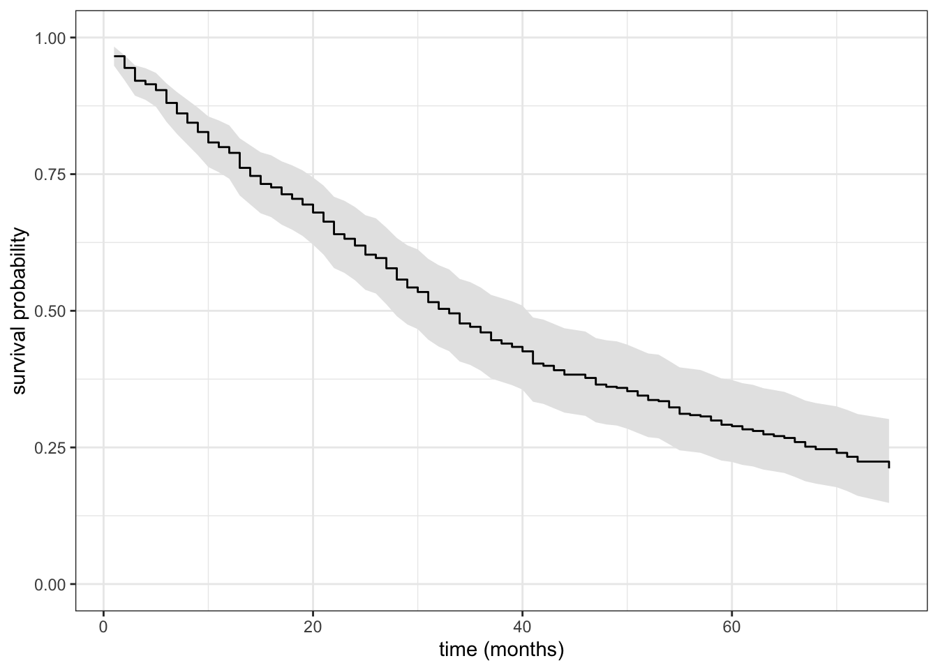
Figure 11.7 shows the Breslow estimate including a pointwise 95% confidence band, which is also computed by the survfit() function. Figure 11.8 shows the fitted survival functions for the four different treatment groups, using the Breslow estimator of the baseline cumulative hazard function, compared to using a Weibull parametric model as baseline. The survival curves are based on the Cox model and in principle computed as \[
\hat{S}_k = e^{-e^{\hat{\beta}_k} \hat{\Lambda}_0}, \quad k = 0, 1, 2, 3.
\tag{11.20}\] Note that for Cox’s proportional hazards model, \(\beta_0 = 0\) always. That is, there is no intercept parameter. Since the baseline hazard is nonparametric, we cannot identify a separate intercept parameter in this model, and the intercept is effectively absorbed into the nonparametric baseline. As pointed out in the survfit() documentation, this also means that there is no such thing as the baseline hazard. What the baseline hazard is depends on a choice of baseline value of \(X\), and thus also on how the predictors are encoded. In this example, the baseline computed by survfit() corresponds to the placebo treatment group, but in more complicated setups the baseline corresponds to a pseudo individual – see ?survfit.coxph.
While it can be instructive to extract the estimated regression parameters and use (11.20) explicitly, the code below used for actually computing the estimated survival functions shown in Figure 11.8 use survfit() with a new dataset, which will give a survival function for each row of the new data. This is both a safer and more convenient way of computing such estimates.
Code
pred_frame <- tibble(
    data = 1:4,
    rx = factor(1:4, labels = levels(prostate$rx)),
    strata = factor(1:4, labels = paste("rx=", rx, sep = ""))
    )
survfit(prostate_cox, newdata = pred_frame) |>
    summary(data.frame = TRUE) |>
    left_join(pred_frame) |>
     ggplot(aes(time, surv, color = strata)) +
        geom_line(data = fit, linetype = 2) +
        geom_step() +
        ylim(0, 1) +
        xlab("time (months)") +
        ylab("survival probability") +
        theme(legend.position = "top")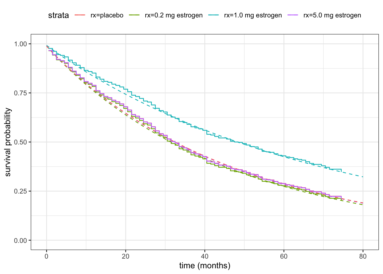
11.4.3 Ties
We did not deal with ties explicitly in any of the derivations in previous sections. If there are ties among the survival times, the summation over \(j: T_i \leq T_j\) in the definition of the cumulative weights is still well defined. If it happens that \(T_i = T_k\) the corresponding cumulative weights \(W_i = W_k\) also become identical. And if both observations are uncensored, they enter into the partial likelihood as the product \[ \frac{w_i}{W_i} \frac{w_k}{W_k} = \frac{w_i w_k}{W_i^2}. \] This implicit way of handling ties is known as Breslow’s method. It treats ties as if they were really due to events that happend at the exact same time.
If the tie \(T_i = T_k\) was due to rounding or grouping, the contribution to the partial likelihood from those two observations should have been one of the two factors: \[ \frac{w_i w_k}{W_i (W_i - w_i)} \quad \text{or} \quad \frac{w_i w_k}{W_k (W_k - w_k)}. \tag{11.21}\]
We could try to break the tie, e.g., by letting the R function order() break ties in whatever arbitrary way it chooses depending on the sorting algorithm and the original order of the data. This naive solution will break all ties but in a unsystematic way, choosing one of the two factors above arbitrarily. Breaking ties in this way appears difficult to justify, and we should probably only break ties if we actually know and use the correct ordering prior to the rounding.
Efron’s method14 represents instead the “correct but unknown” factor by an approximation. Efron’s approximation for two ties is \[ \frac{w_i w_k}{W_i (W_i - (w_i + w_k)/2)} = \frac{w_i w_k}{W_k (W_k - (w_i + w_k)/2)} \] with similar formulas for more than two ties. The approximation is close to the geometric mean of the factors (11.21).
14 The default in coxph() for handling ties is Efron’s method.
Results rarely depend much on whether Efron’s or Breslow’s method (or even naive tie breaking) is used, but Efron’s method is usually preferred if the ties are due to a lack of precision and not to a true discrete nature of the survival times.
11.5 Survival residuals
Model fit can be assessed for survival regression models just as for generalized linear models by means of residuals. There are, of course, several different possible choices.
11.5.1 Cox-Snell residuals
Cox-Snell residuals are not really residuals in a classical sense, but a transformation of the observed survival times to a set of random variables whose distribution should be exponential if the model is correct. They are based on the following result.
Lemma 11.3 If \(T\) has continuous cumulative hazards function \(\Lambda\) then \(\Lambda(T)\) is exponentially distributed with rate 1.
Proof. The survival function \(S(t) = \exp(-\Lambda(t))\) is continuous, whence
\[
S(T) \sim \text{unif}([0,1]).
\] From this it follows that \[
P(\Lambda(T) \leq t) = P(S(t) > \exp(-t)) = 1 - \exp(-t)
\] for \(t \geq 0\), or \(\Lambda(T) \sim \text{Exp}(1)\).
Definition 11.9 With \(\hat{\Lambda}_i\) an estimator of the cumulative hazard function for \(T_i\) the Cox-Snell residuals are defined as \[ \hat{\Lambda}_i(T_i) \tag{11.22}\] for \(i = 1, \ldots, n\).
From the lemma above we conclude that if \((T_1, \delta_1), \ldots, (T_n, \delta_n)\) are independently right censored survival times with corresponding hazard functions \(\Lambda_1, \ldots, \Lambda_n\), then \[ (\Lambda_1(T_1), \delta_1), \ldots, (\Lambda_n(T_n), \delta_n) \] are independently right censored i.i.d. exponentially distributed variables.
If there were no censoring, we would expect the Cox-Snell residuals to follow approximately an exponential distribution. With censoring the Cox-Snell residuals are expected to be approximately independently censored exponentially distributed. We use this in practice by estimating the cumulative hazards function for the Cox-Snell residuals using, e.g., the Nelson-Aalen estimator or the negative log of the Kaplan-Meier estimator. The resulting estimate is then compared to the cumulative hazard for the exponential distribution, which is \(\Lambda(t) = t\). In practice we plot the estimated cumulative hazards against the Cox-Snell residuals, which should fall on a straight line with slope \(1\).
11.5.2 Martingale residuals
The martingale residuals are defined as \[ \delta_i - \hat{\Lambda}_i(T_i), \] and are thus the status indicators minus the Cox-Snell residuals. Their usefulness is partly justified by the following result.
Lemma 11.4 If \(T = \min\{T^*, C\}\) with \(T^*\) and \(C\) having continuously differentiable survival functions it holds that \[ E(\Lambda(T)) = P(T^* \leq C). \]
Proof. Let \(S\) and \(H\) denote the survival functions of \(T^*\) and \(C\), respectively. By integration by parts \[ \begin{align*} E(\Lambda(T)) & = - \int_0^{\infty} \Lambda(t) (SH)'(t) \mathrm{d} t = \int_0^{\infty} \Lambda'(t) S(t) H(t) \mathrm{d} t \\ & = \int_0^{\infty} f(t) H(t) \mathrm{d} t = P(T^* \leq C). \end{align*} \]
The survival function for the minimum of the two independent random variables \(T^*\) and \(C\) is the product \(SH\), whence the density of their distribution is the negative derivative \(-(SH)'\).
It follows from Lemma 11.4 that with \(\delta = 1(T^* \leq C)\) then \[ E (\delta - \Lambda(T)) = 0. \tag{11.23}\] Thus if \(\hat{\Lambda}_i\) were the true cumulative hazards function, the martingale residuals would have mean zero.
Now \(\hat{\Lambda}_i\) is only an estimate, but if the model fits the data, the martingale residuals should have approximately mean \(0\). In the more advanced theory of survival analysis they also enjoy a martingale property, which explains their name. Here we will not pursue this, but just observe that we can investigate the model fit by investigating if the martingale residuals approximately have mean \(0\). The residuals can be used much as regression residuals to judge overall fit as well as the fit of how the individual predictor variables enter into the model. It should be noted, though, that they by definition have a left skewed distribution15 concentrated on \((-\infty, 1)\).
15 The martingale residuals are never approximately normally distributed!
Example 11.12 As for other regression models, we can use augment() from the broom package to extract fitted values (the linear predictor) and residuals. Figure 11.9 shows the martingale residuals plotted against the treatment (which is the only predictor in the model at this point). Since the dataset is rather small, it makes sense here to use geom_beeswarm() from the ggbeeswarm package to visualize the full distribution of the residuals as well as the individual points. Note the upper cap at \(1\) of all martingal residual distributions.
Code
augment(prostate_cox, data = prostate) |>
    ggplot(aes(rx, .resid)) +
    ggbeeswarm::geom_beeswarm(alpha = 0.4) +
    geom_point(
        stat = "summary",
        fun = mean,
        color = "blue",
        size = 2.5
    ) +
    geom_errorbar(
        stat = "summary",
        fun.data = mean_se,
        fun.args = list(mult = 1.96),
        color = "blue",
        width = 0.15,
        linewidth = 0.7
    )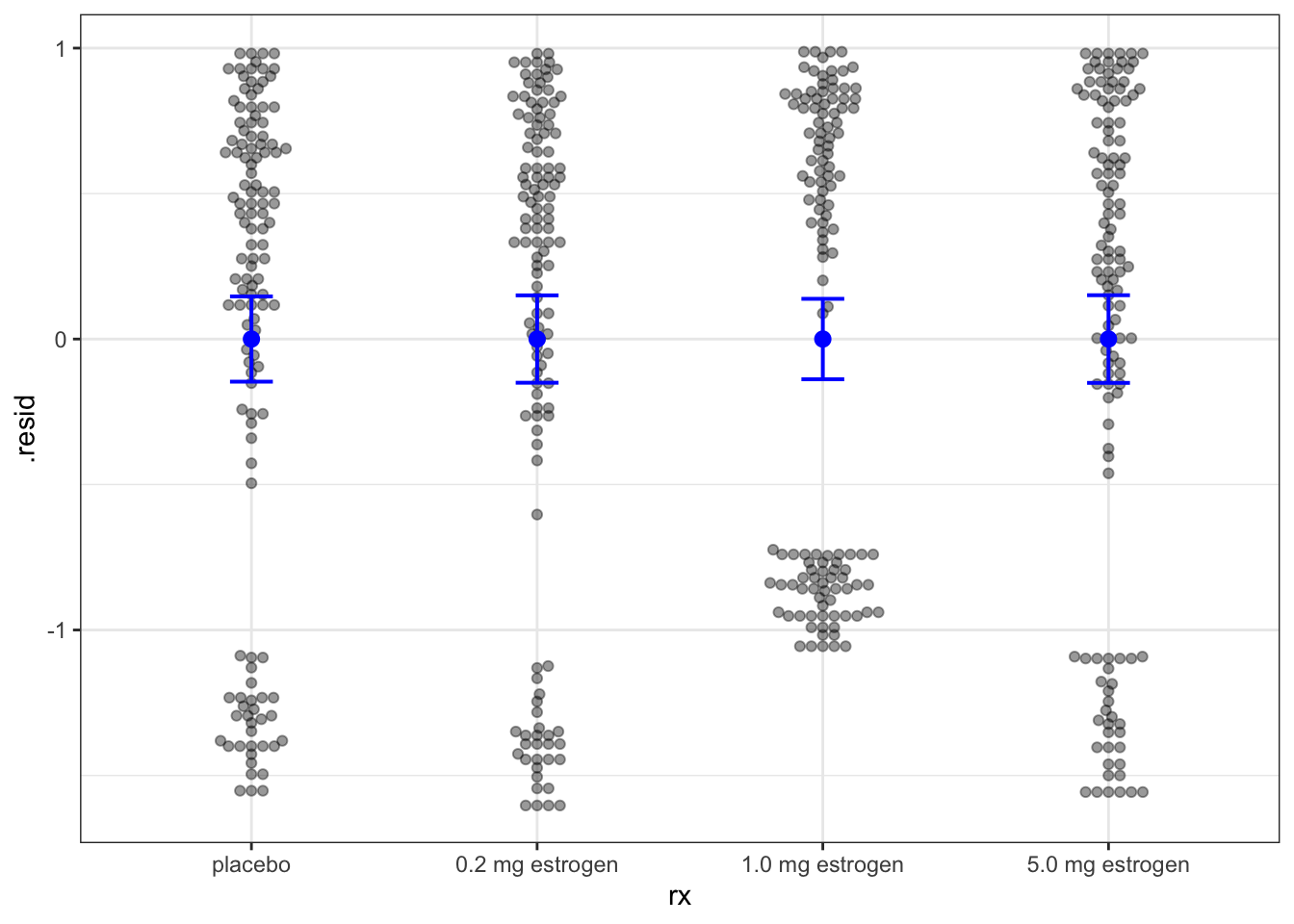
Figure 11.9 includes means and confidence intervals for each group of residuals, which should include zero for all groups as in the figure.
We can also plot the residuals against another potential predictor, such as age, as in Figure 11.10. We see a clear association between age and the residuals suggesting that age (unsurprisingly) holds predictive information about the survival times.
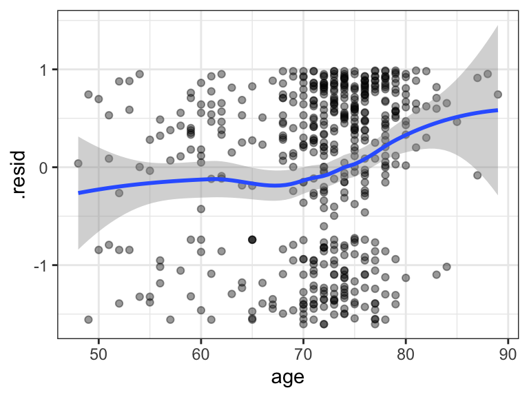
age, which was not included as a predictor in the model.
We want to include age in the model, and we will first try to include it as an additive term.
Code
prostate_cox_add <- coxph(
    Surv(dtime + 0.5, status != "alive") ~ age + rx,
    data = prostate,
)
Figure 11.11 shows two residual plots. One based on comparing the Cox-Snell residuals to the exponential distribution and standard type of a residual plot, this time of the martingale residuals against the fitted values. The fitted values are the linear predictors. For the computation of the Cox-Snell residuals, we used that type.predict = "expected" in the call of augment() gives \(\hat{\Lambda}(T_i)\) as the predicted values (.fitted column in the output).
Code
p1 <- augment(prostate_cox_add, data = prostate, type.predict = "expected") |>
    survfit(Surv(.fitted, status != "alive") ~ 1, data = _) |>
    summary(data.frame = TRUE) |>
    ggplot(aes(time, cumhaz)) +
    geom_abline(slope = 1, color = "blue") +
    geom_point() +
    xlab("Cox-Snell residuals") +
    ylab("Cumulative hazard")


p2 <- augment(prostate_cox_add) |>
    ggplot(aes(.fitted, .resid)) +
    geom_point(alpha = 0.4) +
    geom_smooth() +
    xlab("Fitted values") +
    ylab("Martingale residuals")

gridExtra::grid.arrange(p1, p2, ncol = 2)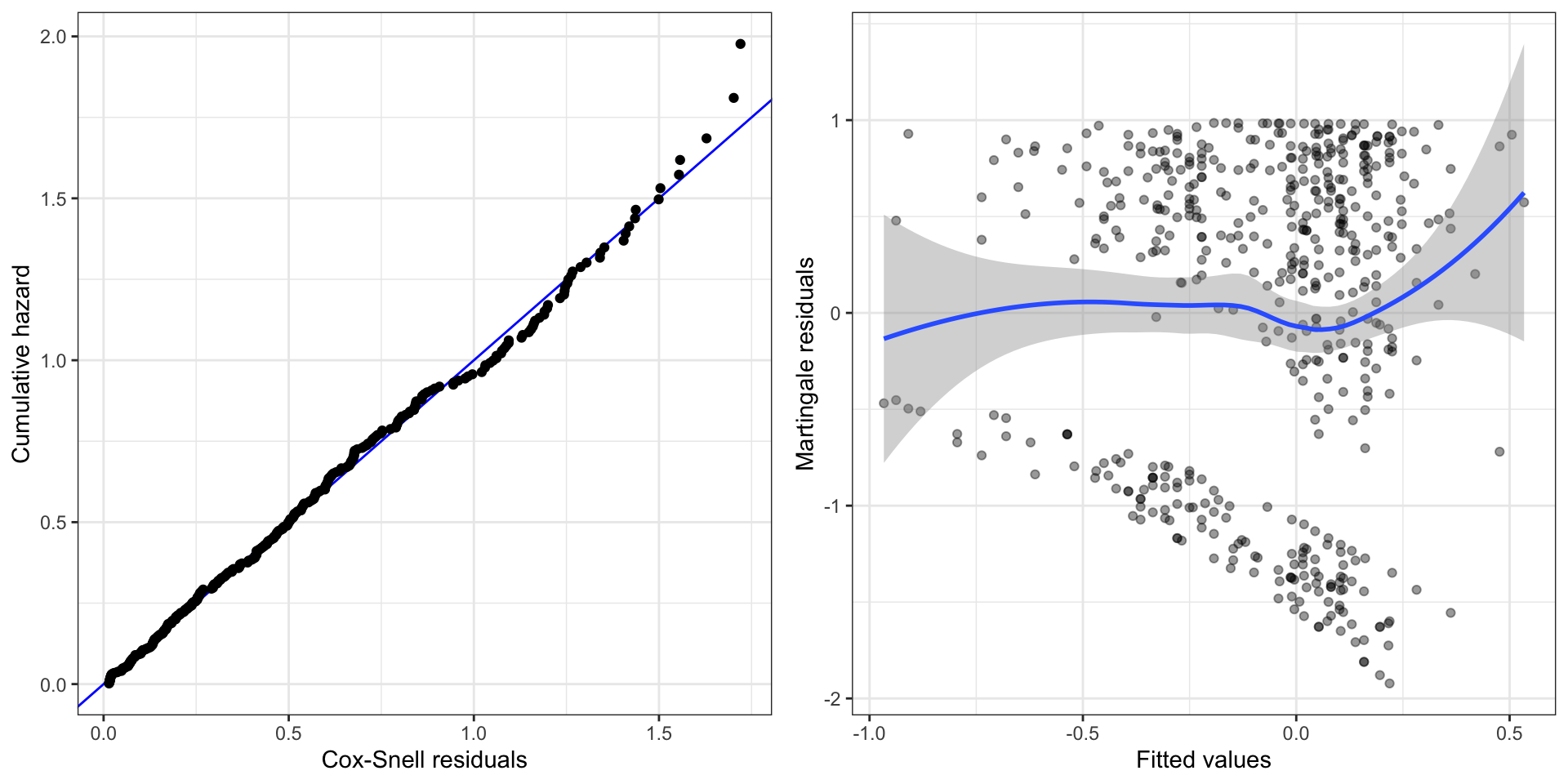
We can see minor model misspecifications from the residual plots in Figure 11.11. First, there are deviations from a straight line in the Cox-Snell plot, suggesting some form of model misspecification. The smoothed curve in the martingale residual plot also suggests some minor model misspecification. We could suspect that age is not correctly modeled.
11.5.3 Deviance residuals
Alternative residuals include the deviance residuals and the Schoenfeld residuals. We will not treat the latter, but the former are based on the following observation. The Poisson nonparametric log-likelihood as well as the parametric log-likelihood with a continuous baseline can be written as \[ \ell^* = \sum_{i=1}^n \underbrace{\delta_i \log (w_i \Lambda_{0,i}) - w_i \Lambda_{0,i}}_{\text{Poisson log-likelihood term}} + \sum_{i=1}^n \delta_i \log \left(\frac{\lambda_{0,i}}{\Lambda_{0,i}}\right) \] The first term is identical to the Poisson log-likelihood, and the second term does not depend on parameters that enter into the weights. Based on this we define the deviance residuals in terms of the Poisson deviances \[ d(\delta_i, \hat{\Lambda}_{i}) = 2\left( \delta_i \log (\delta_i/\hat{\Lambda}_{i}) - \delta_i + \hat{\Lambda}_{i}\right), \] where \(\hat{\Lambda}_{i} = \hat{w}_i \hat{\Lambda}_{0,i}\).
The result is the deviance residuals \[ \text{sign}(\delta_i - \hat{\Lambda}_i) \sqrt{d(\delta_i, \hat{\Lambda}_i)} = \left\{\begin{array}{ll} - \sqrt{2 \hat{\Lambda}_i} & \quad \text{if } \delta_i = 0 \\ \text{sign}( 1 - \hat{\Lambda}_i)\sqrt{ 2( \hat{\Lambda}_i - 1 - \log \hat{\Lambda}_i)} & \quad \text{if } \delta_i = 1 \end{array} \right. \]
Observe that the deviance residuals can be expressed as \[ \text{sign}(\hat{r}_i) \sqrt{-2(\hat{r}_i + \delta_i \log (\delta_i - \hat{r}_i))} \] with \(\hat{r}_i = \delta_i - \hat{\Lambda}_i\) the martingale residuals. Compared to the martingale residuals, the distribution of the deviance residuals is less skewed.
11.5.4 Prostate cancer continued
We conclude this section by a final analysis of the prostate cancer data based on the insights we have obtained from the previous sections. We include both age and treatment rx in the model. Now with age nonlinearly expanded using natural cubic splines and rx interacting (linearly) with age.
Code
prostate_cox_int <- coxph(
    Surv(dtime + 0.5, status != "alive") ~ ns(age, df = 4) + age * rx,
    data = prostate,
)
We first reconsider the residual plots in Figure 11.12. In contrast to Figure 11.11 there are no indications in these residual plots of any model misspecification.
Code
p1 <- augment(prostate_cox_int, data = prostate, type.predict = "expected") |>
    survfit(Surv(.fitted, status != "alive") ~ 1, data = _) |>
    summary(data.frame = TRUE) |>
    ggplot(aes(time, cumhaz)) +
    geom_abline(slope = 1, color = "blue") +
    geom_point() +
    xlab("Cox-Snell residuals") +
    ylab("Cumulative hazard")


p2 <- augment(prostate_cox_int) |>
    ggplot(aes(.fitted, .resid)) +
    geom_point() +
    geom_smooth() +
    xlab("Fitted values") +
    ylab("Martingale residuals")

gridExtra::grid.arrange(p1, p2, ncol = 2)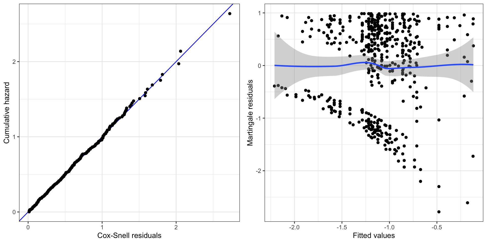
To better understand the interaction model we will compute and visualize the estimated risk factors \[ e^{\hat{\eta}} \] for some combinations of treatment and age as well as the corresponding fitted survival curves.
Code
pred_frame <- expand.grid(
        age = c(55, 62.5, 70, 77.5),
        rx = factor(1:4, labels = levels(prostate$rx))
    )

pred_frame <- mutate(
        pred_frame,
        risk = predict(
            prostate_cox_int,
            newdata = pred_frame,
            type = "risk"
        ),
        risk = risk / risk[1],
        data = 1:16
) | age | rx | risk | data |
|---|---|---|---|
| 55.0 | placebo | 1.000 | 1 |
| 62.5 | placebo | 0.989 | 2 |
| 70.0 | placebo | 0.894 | 3 |
| 77.5 | placebo | 1.313 | 4 |
| 55.0 | 0.2 mg estrogen | 1.438 | 5 |
| 62.5 | 0.2 mg estrogen | 1.231 | 6 |
| 70.0 | 0.2 mg estrogen | 0.963 | 7 |
| 77.5 | 0.2 mg estrogen | 1.224 | 8 |
| 55.0 | 1.0 mg estrogen | 0.391 | 9 |
| 62.5 | 1.0 mg estrogen | 0.499 | 10 |
| 70.0 | 1.0 mg estrogen | 0.582 | 11 |
| 77.5 | 1.0 mg estrogen | 1.102 | 12 |
| 55.0 | 5.0 mg estrogen | 0.494 | 13 |
| 62.5 | 5.0 mg estrogen | 0.679 | 14 |
| 70.0 | 5.0 mg estrogen | 0.852 | 15 |
| 77.5 | 5.0 mg estrogen | 1.738 | 16 |
The computations above give a data frame with estimated risk factors for 16 combinations of age and treatment. Since these factors are always relative risk factors, we have normalized them so that the placebo treatment for age 55 is the reference. Table 11.8 shows the table of the resulting risk factors. Recall that the smaller the risk factor is, the smaller is the risk of dying and the longer is the survival time.
Figure 11.13 shows a plot of the estimated risk factors, from which the nonlinear and non-additive nature of the model is clear. For the high treatment dosage there is a notable change from reducing the risk relative to placebo for patients younger than about 70 years while it increases the risk for the older patients.
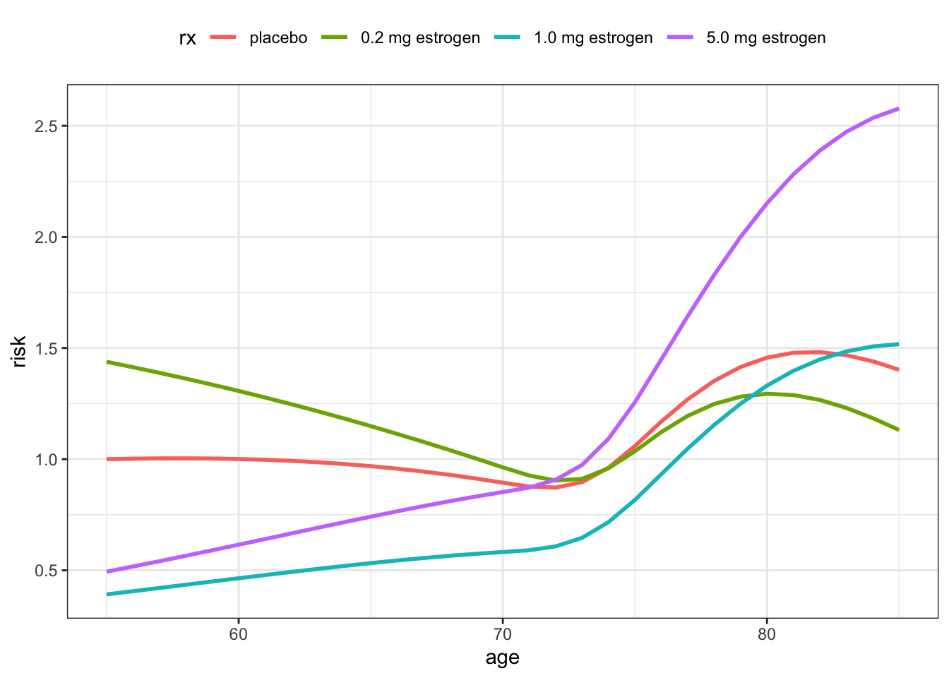
Figure 11.14 shows the fitted survival functions corresponding to the risk factors in Table 11.8. It gives a different perspective on how the estimated survival curves change with age, and how the interaction effect makes the treatment with the high dosage appear beneficial for younger patients while harmful for older patients.
Code
survfit(prostate_cox_int, newdata = pred_frame) |>
    summary(data.frame = TRUE) |>
    left_join(pred_frame) |>
    ggplot(aes(time, surv, color = rx)) +
    geom_step(
        data = summary(prostate_KM, data.frame = TRUE),
        aes(color = NULL),
        linetype = 2
        ) +
    geom_step() +
    facet_wrap("age", ncol = 4) +
    theme(legend.position = "top")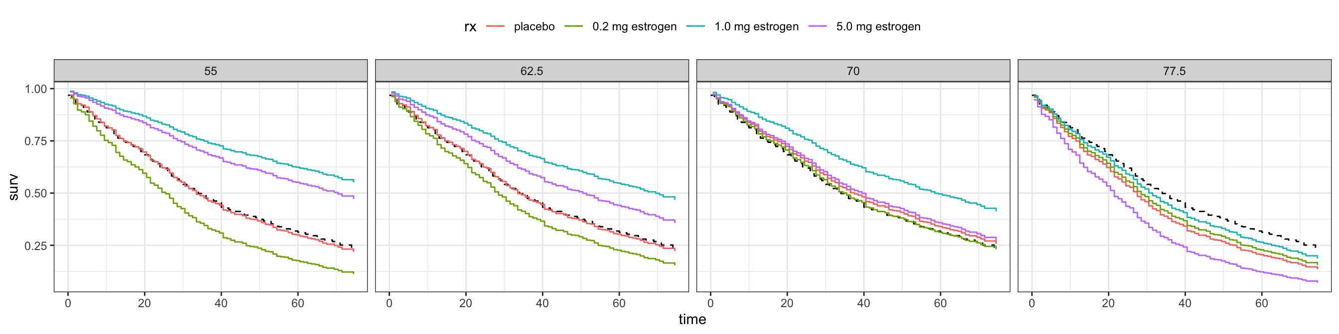
We have not quantified the uncertainty in the above figures. One way to globally test if there is a treatment effect in this interaction model is via a likelihood-ratio test (using the partial likelihood). Table 11.9 shows that the \(p\)-value is about \(0.003\) and thus fairly small. Based on this test we therefore reject the hypothesis that there is no treatment effect.
Code
prostate_cox_age <- coxph(
    Surv(dtime + 0.5, status != "alive") ~ ns(age, df = 4),
    data = prostate,
)
anova(prostate_cox_age, prostate_cox_int) |>
    tidy() |>
knitr::kable()| term | logLik | statistic | df | p.value |
|---|---|---|---|---|
| ~ ns(age, df = 4) | -1999.203 | NA | NA | NA |
| ~ ns(age, df = 4) + age * rx | -1989.345 | 19.7167 | 6 | 0.0031098 |
Today, estrogen treatment of prostate cancer has largely been replaced by better alternatives. Though it is documented to be effective against the cancer, a serious known sideeffect is increased risk of cardiovascular disease. This knowledge is in line with our findings for this particular study.
11.6 Discrete time survival models
We have in previous sections mostly considered survival distributions that are continuous, that is, distributions on \([0, \infty)\) with a continuous survival function \(S\). It was typically even differentiable with \(-S'\) the density of the distribution, in which case the hazard function is well defined. In this chapter we will briefly touch on discrete survival distributions, and almost exclusively on distributions with point masses in the observations \(T_1, \ldots, T_n\). We assume throughout this section that there are no ties.
Definition 11.10 With observations \(T_1, \ldots, T_n\) and \(\rho\) a probability measure on \([0, \infty)\) with survival function \(S\), the empirical likelihood with right censoring is \[ L(\rho) = \prod_i \rho(T_i)^{\delta_i} S(T_i)^{1-\delta_i}. \]
The factors in the empirical likelihood are simply the probabilities \[ \rho(T_i)^{\delta_i} S(T_i)^{1-\delta_i} = P(T^* = T_i, \delta = \delta_i) = \left\{ \begin{array}{ll} P(T^* = T_i) & \quad \text{if } \delta_i = 1 \\ P(T^* > T_i) & \quad \text{if } \delta_i = 0 \end{array} \right. \]
Recall also that for the discrete probability measure \(\rho\), the survival function is \[ S(t) = P(T^* > t) = \sum_{i: T_i > t} \rho(T_i). \] We will show in this section that the Kaplan-Meier estimator can be derived as the maximizer of the empirical likelihood.
11.6.1 Discrete hazards
In the previous section we only introduced hazards for continuous distributions. The discrete hazards are by definition the conditional probabilities \[ \lambda_i \coloneqq \frac{\rho(T_i)}{S(T_i-)} = P(T^* = T_i \mid T^* \geq T_i). \] Note that the discrete hazards are probabilities and thus constrained to lie in the interval \([0,1]\).
Lemma 11.5 For a discrete probability measure with point masses in \(T_1, \ldots, T_n\) and corresponding hazards \(\lambda_i\) the survival function is \[ S(t) = \prod_{i: T_i \leq t} (1 - \lambda_i). \]
Proof. Note that \(S(T_{(j)}-) = S(T_{(j-1)})\) for \(j \geq 2\) and that it is sufficient to show the identity for \(t = T_{(j)}\), \(j = 1, \ldots, n\).
The proof is by induction. For \(T_{(1)}\) we have \(S(T_{(1)}-) = 1\) and \[ S(T_{(1)}) = 1 - \rho(T_{(1)}) = 1 - \lambda_{(1)}, \] which gives the induction start.
For the induction step, observe that the definition of the hazard implies that \[ \begin{align*} S(T_{(j)}) & = S(T_{(j)}-) - \rho(T_{(j)}) \\ & = S(T_{(j)}-) - S(T_{(j)}-)\lambda_{(j)} \\ & = S(T_{(j-1)})(1-\lambda_{(j)}), \end{align*} \] which gives the induction step.
Lemma 11.5 shows that the discrete hazards determine the survival function and thus the distribution, but in a slightly different way than for continuous distributions. As a direct corollary we can express the empirical likelihood in terms of the discrete hazards.
Corollary 11.2 With \(Y_i = Y(T_i) = \sum_{j} 1(T_i \leq T_j)\) the number of individuals at risk at time \(T_i\), the empirical likelihood equals \[ L(\rho) = \prod_{i} \lambda_i^{\delta_i} (1 - \lambda_i)^{Y_i - \delta_i}. \tag{11.24}\]
Proof. From the definition of the hazards and Lemma 11.5 \[ \rho(T_i) = \lambda_i S(T_i-) = \prod_{j: T_j \leq T_i} (1 - \lambda_j). \]
We then plug this expression into the empirical likelihood function and interchange the product order to get \[ \begin{align*} L(\rho) & = \prod_i \lambda_i ^{\delta_i} \prod_{j: T_j < T_i} (1 - \lambda_j)^{\delta_i} \prod_{j: T_j \leq T_i} (1 - \lambda_j)^{1-\delta_i} \\ & = \prod_{i} \lambda_i^{\delta_i} (1 - \lambda_i)^{Y_i - \delta_i}. \end{align*} \]
11.6.2 Empirical likelihood estimators
In terms of the empirical likelihood we define the nonparametric maximum-likelihood estimator (NPMLE) of the survival distribution as the maximizer of \(L\). To compute it we maximize \(L\) as a function of the discrete hazards. To this end we need the following lemma.
Lemma 11.6 With \(y \geq 1\) the function \[ \lambda \mapsto \lambda (1 - \lambda)^{y - 1} \] attains a unique maximum over \([0, 1]\) in \(1/y\).
Proof. With \(f(\lambda) = \lambda (1 - \lambda)^{y - 1}\) we have \[ \begin{align*} f'(\lambda) & = (1 - \lambda)^{y - 1} - \lambda (y-1) (1 - \lambda)^{y - 2} \\ & = (1 - \lambda)^{y - 2}(1 - \lambda - \lambda (y - 1)) \\ & = (1 - \lambda)^{y - 2} (1 - \lambda y). \end{align*} \] For \(y = 1\), the function is the identity, which attains its maximum in \(1 = 1/y\). For \(y > 1\) we have \(f(\lambda) \geq 0\) for \(\lambda \in [0,1]\), \(f(0) = f(1) = 0\) and the function has a unique stationary point in \((0, 1)\) in \(1/y\) with \(f(1/y) > 0\). Thus \(1/y\) is the unique maximizer in \([0,1]\) for \(y \geq 1\).
Theorem 11.2 The NPMLE of the hazards – the hazards for the probability measure that maximizes the empirical likelihood – is given by \[ \hat{\lambda}_i = \frac{\delta_i}{Y_i}. \]
Proof. The factors of \(L\) in (11.24) equal \[ \lambda_i^{\delta_i} (1 - \lambda_i)^{Y_i - \delta_i} = \left\{ \begin{array}{cc} (1-\lambda_i)^{Y_i} & \quad \text{if } \delta_i = 0 \\ \lambda_i (1-\lambda_i)^{Y_i - 1} & \quad \text{if } \delta_i = 1 \\ \end{array} \right. \] In the first case, when \(\delta_i = 0\), the factor is maximized in \(0\), and in the second case, when \(\delta_i = 1\), the factor is maximized in \(1/Y_i\).
By plugging in the NPMLE of the hazards in the formula in Lemma 11.5 for the survival function we find that the NPMLE of the survival function is \[ \hat{S}(t) = \prod_{i: T_i \leq t} \left(1 - \frac{\delta_i}{Y_i}\right). \] We recognize this as the Kaplan-Meier estimator.
In terms of the discrete hazards the corresponding jump cumulative hazard function is \[
\Lambda(t) = \sum_{i : T_i \leq t} \lambda_i.
\] If we plug in the NPMLE of the hazards in this formula, we get \[
\hat{\Lambda}(t) = \sum_{i : T_i \leq t} \frac{\delta_i}{Y_i},
\] which we recognize as the Nelson-Aalen estimator. The previously observed
discrepancy between the Kaplan-Meier and Nelson-Aalen estimators was due to the relation in (11.9) assuming a continuous distribution.
The two main points from this section are:
- The Kaplan-Meier estimator has a justification as a nonparametric maximum-likelihood estimator
- When we use the correct relation between hazards and the survival function for discrete distributions, as given by Lemma 11.5, there is no discrepancy between the Kaplan-Meier and Nelson-Aalen estimators.
11.6.3 The discrete proportional hazards model
It is legitimate to consider the proportional hazards model for discrete probability distributions, and use the empirical likelihood function \(L\) for profiling. Contrary to the derivations in Section 11.4.2, that use the Poisson empirical likelihood, the maximizer is not explicit. Moreover, the proportionality assumption for the discrete model does not really provide an approximation of the proportionality assumption for the continuous model.
The appropriate generalization of the proportional hazards model to the discrete case is actually the model \[ \lambda_i = 1 - (1 - \lambda_{0,i})^{w_i}. \tag{11.25}\]
The empirical likelihood becomes \[ L = \prod_{i} ( 1 - (1 - \lambda_{0,i})^{w_i})^{\delta_i} (1 - \lambda_{0,i})^{W_i - w_i \delta_i}, \] and similar arguments as in the proof of Theorem 11.2 will show that the NPMLE of \(\lambda_{0,i}\) for given weights is \[ \hat{\lambda}_{0,i} = \delta_i\left(1 - \left(1 - \frac{w_i}{W_i}\right)^{1/w_i}\right). \] The corresponding profile likelihood is \[ \prod_{i: \delta_i = 1} \frac{w_i}{W_i} \left(1 - \frac{w_i}{W_i}\right)^{W_i/w_i - \delta_i}. \tag{11.26}\]
The discrete proportional hazards model (11.25) is arguably the “correct” generalization of the continuous proportional hazards model, see Jacobsen (1984), and using the empirical likelihood yields the profile likelihood (11.26). The resulting profile likelihood is not Cox’s partial likelihood, but it is for most practical purposes very close. In the literature, Cox’s partial likelihood has caught on as the default choice for semiparametric estimation of parameters that enter the weights.
Jacobsen, Martin. 1984. “Maximum Likelihood Estimation in the Multiplicative Intensity Model: A Survey.” International Statistical Review 52 (2): 193–207.
Exercises
Exercise 11.1 Show that if \(T\) has a log-logistic distribution with density \(f = f_0\) then \[ e^{\eta} T \] has density \(f_{\eta}\). Show that if \(T\) has a log-logistic distribution with density \(f_{\eta}\) then \[ \log T - \eta \] has a logistic distribution.
Exercise 11.2 Show that without censoring then the Kaplan-Meier estimator equals the empirical survival function \[ \hat{S}(t) = \frac{1}{n} \sum_{i=1}^n 1(T^*_i > t). \]
Exercise 11.3 In this exercise you should consider the prostate dataset from the RwR package and this time include the variable hx in the analysis. The variable hx indicates if the patient has a history of cardiovascular disease. You should ignore the treatment variable rx.
- Fit a proportional hazards model using the two variables
ageandhxas predictors. - Make one or more residual plots for the model you have fitted. Does it fit the data?
- Test the hypothesis that survival is not associated with
hxgivenage.
Exercise 11.4 Let \(T_1^*, \ldots, T^*_n\) be independent survival times for \(n\) patients and let \(X_i \in \{0, 1\}\) indicate if the \(i\)-th patient is treated \((X_i = 1)\) or untreated \((X_i = 0).\) We are interested in estimating the treatment effect, which we summarize in the following parameter of interest \[ \rho := \frac{\text{median}(T_1^* \mid X_1 = 1)}{\text{median}(T_1^* \mid X_1 = 0)}, \] that is, \(\rho\) is the ratio of the median survival time for treated vs. untreated patients.
In this exercise it is assumed that \(T_i^*\) follows a Weibull distribution with shape parameter \(\gamma > 0\) and scale parameter \(\alpha_{x_i}\), that is, the hazard rate is \[ \lambda_i(t) = \alpha_{x_i} \gamma t^{\gamma-1}. \]
Show that \[ \rho = \sqrt[\gamma]{\frac{\alpha_0}{\alpha_1}} \] in terms of the Weibull parameters.
Show that the Weibull model can be formulated as a proportional hazard model in terms of the linear predictor \[ \eta_i = \beta_0 + \beta_1 X_i \] and relate the parameters \(\beta_0\) and \(\beta_1\) to \(\alpha_0\) and \(\alpha_1\). Express \(\rho\) in terms of the \(\beta_0\) and \(\beta_1\) parameters.
In the remaining part of this exercise we will study two different estimators of \(\rho\) on simulated data. To this end introduce i.i.d. censoring times \(C_1, \ldots, C_n\) and the censored observed survival times \[ T_i = \min\{T_i^*, C_i\}. \]
The data set testWei available from the R package RwR is a simulated data set with \(n = 200\), \(X_1 = \ldots = X_{100} = 0\) and \(X_{101} = \ldots = X_{200} = 1\), with \(\gamma = 2\), \(\beta_0 = 0\) and \(\beta_1 = -1\) (so that \(\rho \approx 1.649\)). The censoring times are uniformly distributed on \([0, 4]\). The time column contains the \(T_i\)-s and the status column is the indicator of censoring (\(1\) is uncensored, \(0\) is censored).
Compute and plot the Kaplan-Meier estimates of the survival function within each of the two treatment groups for the simulated
testWeidata set.Use the Weibull model with fixed \(\gamma = 2\) to estimate \(\beta_0\) and \(\beta_1\). Compare the resulting estimated survival functions from the Weibull model with the Kaplan-Meier estimates.
Compute the MLE \(\hat{\rho}_{\mathrm{MLE}}\) of \(\rho\) based on the Weibull model (with fixed \(\gamma = 2\)) and compute a 95% confidence interval for \(\rho\). Compute also, based on the Kaplan-Meier estimates, a direct estimate, \(\hat{\rho}_{\mathrm{KM}}\), of \(\rho\).
Write an R program that simulates a data set (including the censoring) using the same setup as for the
testWeidata set described above. Simulate \(B = 200\) data sets and compute for each data set the estimates \(\hat{\rho}_{\mathrm{KM}}\) and \(\hat{\rho}_{\mathrm{MLE}}\) as above and compare their distributions.
Hint: Use the R function rweibull() to simulate from the Weibull distribution, but pay attention to the parametrization.
Exercise 11.5 For this exercise we consider the data set lung on lung cancer survival available from the R package RwR. It contains four variables:
| Variable | Description |
|---|---|
| time | survival time in days |
| status | censored = 1, dead = 2 |
| age | age in years |
| sex | male = 1, female = 2 |
- Plot the Kaplan-Meier estimates of the survival functions for males and females separately.
- Use the Cox proportional hazard model to investigate if the survival time depends upon age.
- Check if the Cox proportional hazard model fits the data.
Exercise 11.6 This exercise is about the proportional hazard model with cumulative hazard function \[ \Lambda_i(t) = e^{\eta_i} \Lambda_0(t) \] for the \(i\)-th individual and linear predictor \[ \eta_i = \beta_0 + \beta_{\texttt{age}} X_{i, \texttt{age}} + \beta_{\texttt{sex}} X_{i, \texttt{sex}}. \] Thus the two predictor variables are the age and sex of the individual.
You will need that data set simSurv from the R package RwR that contains the four variables, surv, status, age and sex being the censored survival times, the censoring indicator, the age and the indicator of gender (1 is male), respectively, of the individuals. There is a total of 200 individuals.
- Estimate, using Cox’s proportional hazard model, the parameters \(\beta_{\texttt{age}}\) and \(\beta_{\texttt{sex}}\). Compute a 95% confidence interval for \(\beta_{\texttt{sex}}\) and determine whether males have a higher risk of dying than females.
For the remaining questions the baseline cumulative hazard function is assumed to be \[ \Lambda_0(t) = e^{\gamma t} - 1, \quad t \geq 0. \] The cumulative hazard function for the \(i\)-th individual is thus \[ \Lambda_i(t) = e^{\eta_i} ( e^{\gamma t} - 1). \]
We assume that we have independent censored observations \((T_1, \delta_1), \ldots, (T_n, \delta_n)\) with \(T_i \geq 0\) the \(i\)-th censored survival time and \(\delta_i\) the indicator of whether the \(i\)-th observation is censored.
Compute the baseline hazard rate \(\lambda_0(t)\) and show that the log-likelihood function is \[ \sum_{i} \delta_i \eta_i + \delta_i \log (e^{\gamma T_i} - 1) - e^{\eta_i} (e^{\gamma T_i} - 1) + \delta_i \log \frac{\gamma e^{\gamma T_i}}{e^{\gamma T_i} - 1}. \]
Plot the profile log-likelihood for the \(\gamma\)-parameter. Compute the MLE of \(\gamma\), \(\beta_0\), \(\beta_{\texttt{age}}\) and \(\beta_{\texttt{sex}}\).
Hint: Identify the first two terms of the log-likelihood as the log-likelihood for a Poisson generalized linear model. Use the glm()-function for the profiling.
- Use the glm framework to compute a 95% confidence interval for \(\beta_{\texttt{sex}}\) by plugging in the MLE, \(\hat{\gamma}\), of \(\gamma\) and pretending that it is fixed and known. Compute next a 95% confidence interval using non-parametric bootstrapping. Compare the results.
Exercise 11.7 This exercise deals with the numerical algorithms associated with the optimization of Cox’s partial likelihood. Consider censored survival data \((T_i, \delta_i, X_i)\) for \(i = 1, \ldots, n\) with \(T_i\) the possibly censored survival time, \(\delta_i\) the indicator of whether \(T_i\) is uncensored, and \(X_i \in \mathbb{R}\) a univariate real valued predictor. The proportional hazard model is given by the individual weights \[ w_i = e^{\beta X_i} \] for an unknown parameter \(\beta\). In the following we will make the assumption that the survival times are ordered and with no ties, that is \[ T_1 < T_2 < \ldots < T_n. \]
- Show that Cox’s partial log-likelihood equals \[ \ell(\beta) = \sum_{i: \delta_i = 1} \beta X_i - \log \left(\sum_{j \geq i} e^{\beta X_j} \right), \] and compute the first and second derivative of \(\ell\) w.r.t. \(\beta\).
The estimator \(\hat{\beta}\) is the maximizer of \(\ell\) provided that \(\ell\) attains a maximum. It then solves the equation \[ \ell'(\beta) = 0. \]
- Show that \(\ell\) is concave. Find a condition on the \(X_i\)-s that ensure that \(\ell\) has a unique maximum.
For the remaining part of this problem you first need to simulate a data set from the model above. You may experiment with different choices of \(\beta\), but try also \(\beta = 0\).
- Implement Newton’s algorithm for computing \(\hat{\beta}\). Apply the algorithm with start value \(\beta_{1} = 0\) to the simulated data set and investigate the values of \(\beta_m\), \(\ell(\beta_m)\), \(\ell'(\beta_m)\) and \(\ell''(\beta_m)\) in the iterations of the algorithm.
A naive implementation of the computation of e.g. \(\ell\) scales like \(n^2\). Make sure that your implementation scales like \(n\).
Compute and plot an estimate of the baseline cumulative hazard function.
Compute \(\hat{\beta}\) using the
coxph()function in R. Compute also a standard 95% confidence interval for \(\beta\). Compare this interval with a (partial) likelihood interval based on \(\ell\).
Exercise 11.8 This exercise is on theoretical properties of the survival analysis martingale residuals. Let \(T^*\) and \(C\) be independent random variables on \([0,\infty)\), whose distributions have continuous densities \(f\) and \(g\), respectively. The corresponding survival functions are denoted \(S\) and \(H\). Note that \(f = - S'\) and \(g = - H'\). Then \(T = \min\{T^*, C\}\) denotes the observed (censored) survival time and \(\delta = 1(T^* \leq C)\) is the status indicator.
- Show that for any function \(K: [0,\infty) \times \{0,1\} \to \mathbb{R}\), continuously differentiable in the first variable, it holds that \[ \begin{align*} E( K(T, \delta)) & = \int_0^\infty \Big(K(0,1) + (K(s, 0) - K(s,1)) S(s) \\ & \quad + \int_0^s \partial_tK(t, 1) S(t) \mathrm{d} t \Big) g(s) \mathrm{d} s \end{align*} \] provided that the expectation is well defined. Use this to show that16 \[ E (\delta - \Lambda(T)) = 0 \qquad \text{and} \qquad V(\delta - \Lambda(T)) = E(\Lambda(T)) \] where \(\Lambda\) denotes the cumulative hazard function for the distribution given by \(f\).
16 That the expectation is \(0\) is derived in the main text, but a slightly different derivation is provided here. The variance formula is new.
Recall that for the proportional hazard model, the \(i\)-th individual has cumulative hazard function \(w_i \Lambda_0\) where \(w_i\) is an individual weight and \(\Lambda_0\) is the baseline hazard.
Assume that \(\hat{w}_i\) is the estimate of the \(i\)-th weight and that \(\hat{\Lambda}_0\) is the estimate of the baseline. With \(\hat{\Lambda}_i = \hat{w}_i \hat{\Lambda}_0(T_i)\) the fitted cumulative hazard function for the \(i\)-th individual evaluated in \(T_i\), \[ \hat{r}_i = \delta_i - \hat{\Lambda}_i \] is the \(i\)-th martingale residual. Let \(\hat{d}_i\) denote the \(i\)-th deviance residual17.
17 The deviance residuals are sometimes regarded as distribution stabilized transforms of the martingale residuals. This exercise gives some insight on this perspective.
- Give an argument for considering the following standardization of the martingale residuals: \[ \tilde{r}_i = \frac{\hat{r}_i}{\sqrt{\hat{\Lambda}_i}}. \]
- Show that if \(\delta_i = 1\) then \[ \hat{d}_i^2 = \tilde{r}_i^2 + o((1 - \hat{\Lambda}_i)^2). \]
- Explore graphically how good the approximation \[ \hat{d}_i \approx \tilde{r}_i \] is as a function of \(\hat{\Lambda}_i\) when \(\delta_i = 1\). Does a similar approximation hold if \(\delta_i = 0\)?