9  Model Assessment

Warning

This chapter is still a draft and minor changes are made without notice. Some changes to Section 9.6 are to be expected.

This chapter deals with general statistical methodology for assessment of a regression model’s predictive strength. Quantification of predictive strength can be useful in itself for a single model but is most often used for comparing models and for selecting among several models.

It is important to be very clear about the terminology that is used in relation to model assessment. That a model fits the data means throughout that the model assumptions are fulfilled, and goodness-of-fit-measures are quantifications of deviations from the model assumptions. In this chapter the quality of a model is quantified in terms of its predictive strength and not in terms of its fit to data. For a model to be a good predictive model it is neither necessary nor sufficient¹ that it fits the data.

¹ Is this surprising?

9.1 Outline and prerequisites

The chapter first introduces a simple example where temperature is used as a predictor for the number of bikes that a bike sharing company is renting out. Then we present the general theoretical framework of loss and risk for quantification of predictive strength. Subsequently a number of prediction error quantities and corresponding estimators are treated in Section 9.4, where we also return to the bike renting example. The different estimators of prediction error are compared in a simulation study in Section 9.5, and the chapter concludes with some specific results for binary responses.

The chapter primarily relies on the following R packages.

library(RwR)
library(tibble)
library(ggplot2)
library(splines)
library(dplyr)

9.2 Bike rentals

The bike dataset is included in the RwR package. It is a tibble with data from 50 days (50 rows) on the number of bikes rented from a bike sharing company in a day and the average temperature of the day.

# RwR version >= 0.3.2
data("bike", package = "RwR")

Count	Temperature
113	20.555556
40	2.222222
70	28.333333
104	15.555556
129	22.777778
79	10.555556

Table 9.1: First six rows in the bike dataset.

Figure 9.1: Scatter plot of number of rented bikes against temperature.

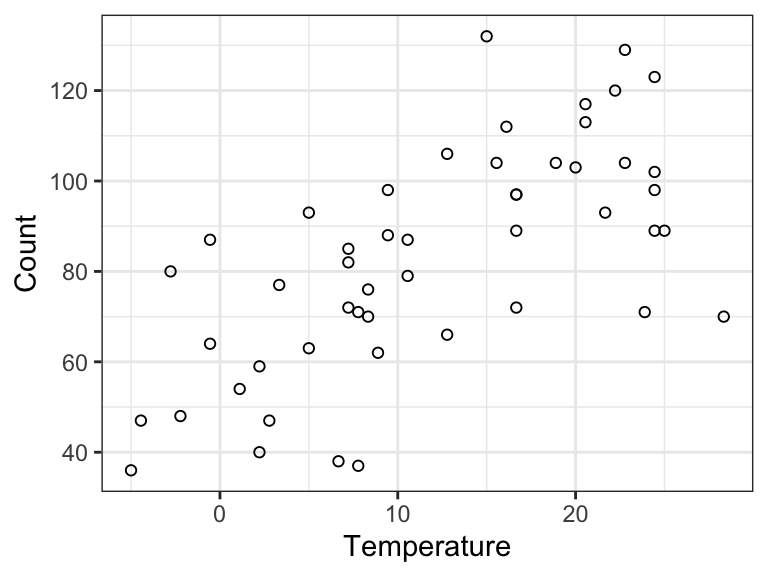
Figure 9.1 shows a scatter plot of the data. We will build a sequence of predictive models of Count using Temperature as the predictor. That is, the response variable \(Y\) is the number of bikes rented and \(X\) is the temperature. All the models are of the form \[ m(x) = E(Y | X = x) = \beta_0 + \sum_{d = 1}^{\mathrm{df}} \beta_d h_d(x) \] where the \(h_d\)-s are spline basis functions. The number \(\mathrm{df}\) specifies the number of basis functions and thus the complexity of the model. The dimension of the corresponding linear model will be \(\mathrm{df} + 1\), since the model also includes an intercept. The code below fits six models for \(\mathrm{df}\) ranging from \(0\) to \(16\).

bike_lm <- list()
df <- c(0, 1, 2, 4, 8, 16)
bike_lm[[1]] <- lm(Count ~ 1, data = bike)
for (d in seq_along(df[-1]) + 1) {
    bike_lm[[d]] <- lm(Count ~ ns(Temperature, df = df[d]), data = bike)
}

Figure 9.2 shows predictions from the six fitted models. We see that as we increase the complexity of the model, the predictions show more and more fluctuations.

p0 <- ggplot(bike, aes(Temperature, Count)) + geom_point(pch = 1) 
plot_pred <- function(pred_data) {
    p0 + geom_line(data = pred_data, aes(y = .predict), linewidth = 1)
}
pred_data <- tibble( 
    Temperature = seq(min(bike$Temperature), max(bike$Temperature), length = 200)
)
p <- list()
for (d in seq_along(df)) {
    p[[d]] <- mutate(
                pred_data, 
                .predict = predict(bike_lm[[d]], newdata = pred_data)
            ) |> plot_pred() + ggtitle(paste("df =", df[d])) 
}
gridExtra::grid.arrange(p[[1]], p[[2]], p[[3]], p[[4]], p[[5]], p[[6]], ncol = 3)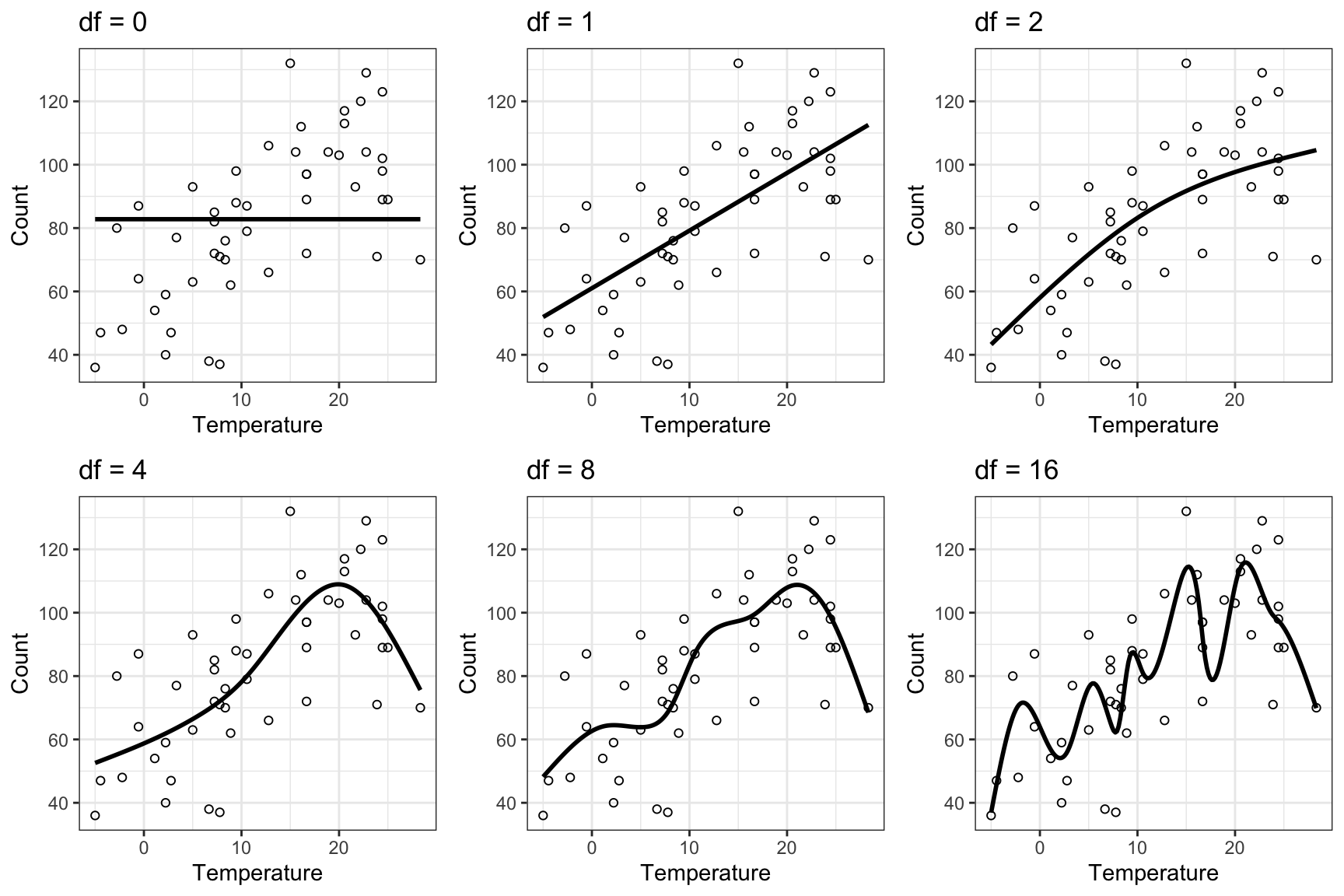

Figure 9.2: Scatter plot of data with model predictions from the six models of bike rentals.

df	MSE	adj r-sq
0	602.1600	0.0000000
1	333.4333	0.4347352
2	320.3021	0.4454431
4	262.9248	0.5245518
8	251.1411	0.5015540
16	195.7884	0.5172112

Table 9.2: Mean squared error on data used to fit the models for the six models of bike rentals.

Table 9.2 shows the adjusted \(R^2\) together with the mean squared error on the data used to fit the models, which is computed as \[ \frac{1}{n} \sum_{i=1}^n (Y_i - \hat{m}(X_i))^2, \tag{9.1}\] where \(\hat{m} = \hat{\beta}_0 + \sum_{d=1}^{\mathrm{df}} \hat{\beta}_d h_d\). We note that the MSE is monotonely decreasing as a function of the complexity of the model, that is, as a function of \(\mathrm{df}\). The adjusted \(R^2\) increases until \(\mathrm{df} = 4\), and then it appears to settle just above \(0.5\) – suggesting that the models can explain around 50% of the variation in the data.

Figure 9.3 shows the residual plots for the six models. We see that the three models with \(\mathrm{df} \leq 2\) are misspecified. This is particularly pronounced for the intercept-only model (\(\mathrm{df} = 0\)). From the residual plots alone, the remaining three models appear to fit the data well.

p <- list()
for (d in seq_along(df)) {
    p[[d]] <- broom::augment(bike_lm[[d]], data = bike) |> 
        ggplot(aes(Temperature, .resid)) + 
        geom_point(pch = 1) + geom_smooth() +
        xlab("") + ylab("") + ggtitle(paste("df =", df[d])) +
        ylim(-50, 50)
}
gridExtra::grid.arrange(p[[1]], p[[2]], p[[3]], p[[4]], p[[5]], p[[6]], ncol = 3)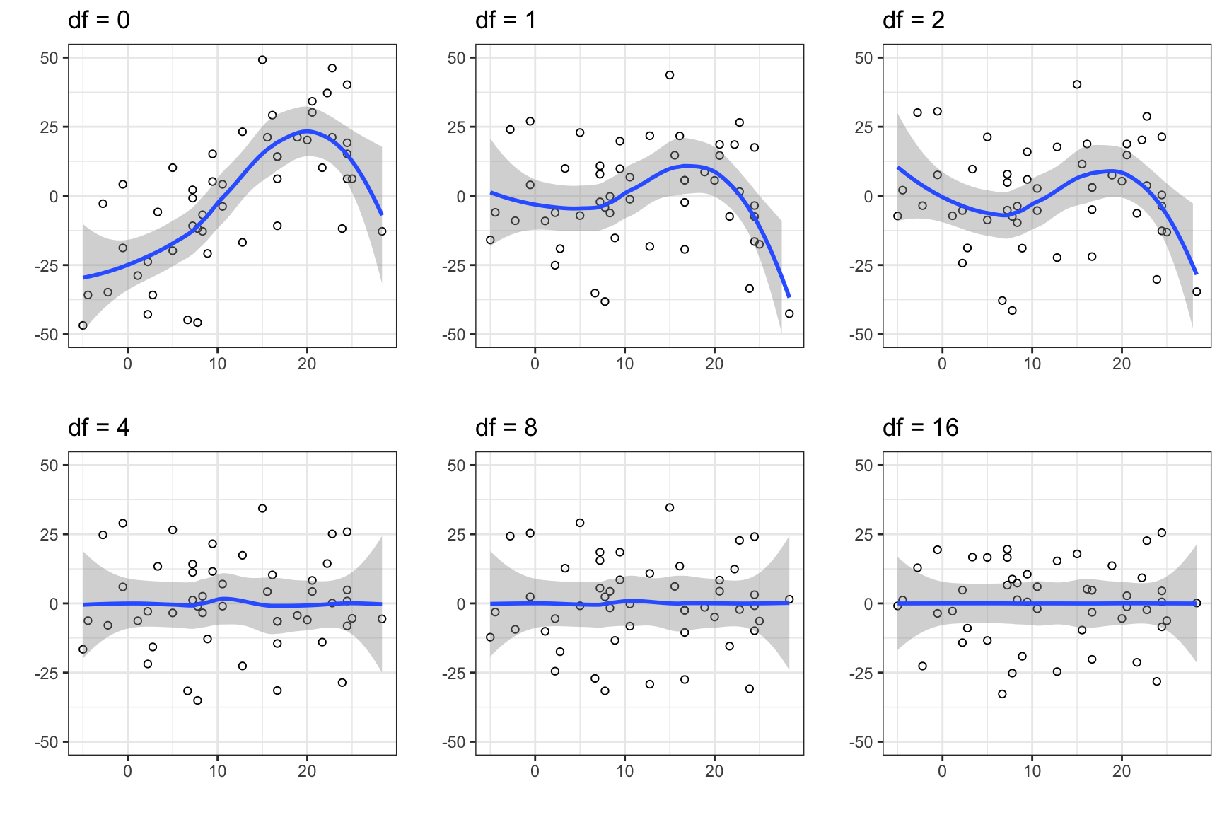

Figure 9.3: Residual plots for the six models of bike rentals.

Based on the MSE in Table 9.2 the most complex model is best. However, the adjusted \(R^2\) suggests that all the three models with \(\mathrm{df} = 4\), \(\mathrm{df} = 8\) and \(\mathrm{df} = 16\) are about equally good, and the residual plots suggest that these three models all fit the data. If we consider the predictions made by the most complex model (\(\mathrm{df} = 16\)) in Figure 9.2, we are probably a little wary about the oscillations of the estimated mean value function. These seem arbitrary and unlikely to generalize to future observations. And by referring to some form of principle of parsimony we can argue that the model with \(\mathrm{df} = 4\) is “best”. It is as complex as it needs to be but not more complex than that. In this chapter we will develop a precise framework for assessing and comparing models, which clarifies what we mean by a model’s predictive performance. We can regard this as a substantiation and clarification of the principle of parsimony that we will adhere to.

9.3 Quantifying model predictions

How do we then quantify the predictive strength of a model? We may already suspect that the empirical MSE, as computed in the bike rental example, is not a good measure. Now MSE is a sensible theoretical quantification, but the empirical MSE given by (9.1) is an example of a training error, as defined in Section 9.4, which is generally a bad estimate of MSE. Alternatives include the adjusted \(R^2\)-statistic, as introduced in Section 2.7, and its equivalents for generalized linear models expressed in terms of either the \(\chi^2\)- or deviance statistic as introduced in Section 6.4. As discussed there, these quantities are measures of the descriptive or predictive strength of a model, but they may appear ad hoc, and we have not dealt with their theoretical properties.

This section deals more systematically with the question of assessing models in terms of their predictive performance by defining various quantifications of a model’s predictive strength. In the subsequent sections we treat methods for correct estimation of these quantities. This section is largely theoretical, and its purpose is to make the conceptual framework for quantifying predictive strength clear. We will, in particular, clarify how the likelihood (or deviance) for exponential dispersion distributions is related to measures of predictive strength, and how the deviance can be seen as a natural generalization of the squared error.

9.3.1 Loss and risk

The predictive strength of a model for predicting \(Y\) is a quantification of the concordance between \(Y\) and the prediction of the model. Before introducing a general approach for making such a quantification a motivating example is considered.

Figure 9.4: The mean squared error is a quadratic function of \(\mu\), which can be decomposed as a sum of the the variance and the squared bias.

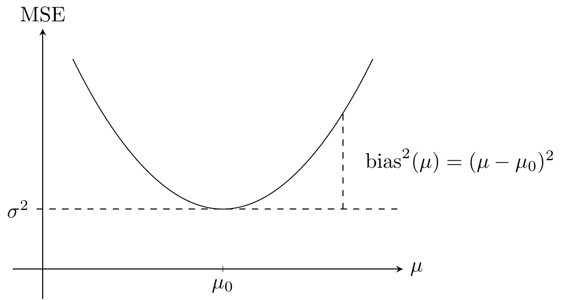
Example 9.1 Assume that \(Y\) is a real valued random variable and that we use the point prediction² \(\mu \in \mathbb{R}\) of \(Y\). Just as the squared error can be used for fitting the model to data it can be used for quantifying predictive strength. Thus \[ \mu \mapsto (Y - \mu)^2 \] is a quantification of how good a prediction \(\mu\) is of \(Y\). Its expectation is the mean squared error \[ \mathrm{MSE}(\mu) = E (Y - \mu)^2. \] If \(\mu_0 = E(Y)\) denotes the mean of \(Y\) and \(\sigma^2 = V(Y)\) its variance then \[ \mathrm{MSE}(\mu) = (\mu_0 - \mu)^2 + E (Y - \mu_0)^2 = \mathrm{bias}^2(\mu) + \sigma^2. \tag{9.2}\] It is clear from (9.2) that the mean squared error is bounded below by \(\sigma^2\) – that does not depend upon \(\mu\) – and that the optimal predictor from a mean squared error perspective minimizes the squared bias term and is equal to \(\mu_0\).

² A point prediction is a single element in the sample space for \(Y\). Alternatives include interval predictions – and probabilistic predictions as introduced below.

In a regression context the prediction \(\mu\) would depend on \(X\), and the mean \(\mu_0\) and the variance \(\sigma^2\) would be conditional on \(X\).

The size of the squared bias can best be interpreted relative to the variance \(\sigma^2\), and the unitless quantity \[\frac{\mathrm{bias}^2(\mu)}{\sigma^2}\] is therefore a useful quantification of the predictive strength of \(\mu\).

A general method for quantifying predictive strength of a probability model is introduced below by replacing the squared error with an arbitrary loss function. The mean squared error is then replaced by a general quantity called the risk. The convention is that a loss function quantifies how discordant predictions and observations are, whereas a reward function quantifies concordance. The negative of a reward function can always be used as a loss function and vice versa, so we will only treat loss functions. The focus in this chapter is mostly on the negative log-likelihood loss, for which the risk is also known as (twice) the cross-entropy, and where it has a decomposition similar to the bias-variance decomposition above.

A point prediction as in Example 9.1 may not in all cases be the most relevant kind of prediction. If \(Y\) is a binary variable, say, it is more informative to make a prediction of the probability that \(Y = 1\) than just predicting that \(Y\) will be \(0\) or \(1\). This is particularly true if \(P(Y = 1)\) is small, in which case the only sensible point prediction of \(Y\) is \(0\). A probabilistic prediction of \(Y\) is simply a probability measure \(\rho\), and to quantify how well \(\rho\) predicts \(Y\) we need to quantify the discordance between \(Y\) and \(\rho\) – or perhaps rather the discordance between the distribution of \(Y\) and \(\rho\).

For the quantification of the discordance we choose a (sensible) loss function \[ (y, \rho) \mapsto \mathrm{Loss}(y, \rho) \in \mathbb{R}. \] Then \(\mathrm{Loss}(Y, \rho)\) quantifies how well \(\rho\) predicts the random variable \(Y\). It is common to also call a loss function used for probabilistic predictions a scoring rule.

Letting \(\rho_0\) denote the distribution of \(Y\), the risk³ of \(\rho\) is the expectation of the loss, \[ \mathrm{Risk}(\rho) = E \big( \mathrm{Loss}(Y, \rho) \big) = \int \mathrm{Loss}(y, \rho) \rho_0(\mathrm{d}y), \] provided that the expectation exists. The larger the value of the loss is, the greater is the discordance, but there is no convention on the scale. Low risk is better than high risk, but the risk of a model can only be interpreted relative to the risk of other models.

³ The loss and risk terminology relates to economic decision theory, but there is no direct monetary interpretation of these quantities in this statistical context. For probabilistic predictions the risk is also known as the expected score.

Definition 9.1 If \(\rho = h \cdot \nu\) has density \(h\) w.r.t. \(\nu\) the negative log-likelihood⁴ loss is \[ \mathrm{Loss}(y, \rho) = - 2 \log h(y). \tag{9.3}\]

⁴ The convention is that \(\log(0) = -\infty\).

The factor “2” in (9.3) is an arbitrary convention, but it aligns with the scaling of the deviance and results in an unscaled squared error loss for the standard normal distribution.

There is an arbitrariness in the choice of \(\nu\) that makes the absolute value of the negative log-likelihood impossible to interpret, but it is suitable for comparisons between two or more probability distributions that all have densities w.r.t. the same measure \(\nu\). This is particularly clear if we compare \(\rho\) to the distribution of \(Y\) – if this distribution has density w.r.t. \(\nu\) as well. To this end we introduce the entropy of the distribution of \(Y \sim \rho_0 = h_0 \cdot \nu\) as \[ H(\rho_0) = - E(\log h_0(Y)) = - \int \log h_0(y) \rho_0(\mathrm{d}y), \] provided that \(\log h_0\) is \(\rho_0\)-integrable.

The entropy introduced here is related to Shannon’s entropy and information theory rather than thermodynamics.

Lemma 9.1 Assume that \(Y \sim \rho_0 = h_0 \cdot \nu\) with entropy \(H(\rho_0)\). Then the risk for the negative log-likelihood loss fulfills \[ \mathrm{Risk}(\rho) \geq 2 H(\rho_0) \tag{9.4}\] for any probability measure \(\rho = h \cdot \nu\) with \(\log h\) being \(\rho_0\)-integrable. Moreover, the inequality in (9.4) is sharp unless \(\rho = \rho_0\).

Proof. First note that \(- E(\log h(Y)) = - \int \log h(y) \rho_0(\mathrm{d}y).\) Introducing the set \(A = \{y \mid h_0(y) > 0\}\) with \(\rho_0(A) = 1\) and the function \[ r(y) = \left\{\begin{array}{ll} \frac{h(y)}{h_0(y)} & \quad \mathrm{for } \ y \in A \\ 1 & \quad \mathrm{for } \ y \not \in A \end{array}\right. \] we find that \[ \begin{align*} \frac{1}{2} \mathrm{Risk}(\rho) - H(\rho_0) & = - \int \log h(y) \rho_0(\mathrm{d} y) + \int \log h_0(y) \rho_0(\mathrm{d} y) \\ & = \int_A -(\log h(y) - \log h_0(y)) \rho_0(\mathrm{d} y) \\ & = \int_A - \log r(y) \rho_0(\mathrm{d}y) \\ & = \int - \log r(y) \rho_0(\mathrm{d}y). \end{align*} \] Since the negative logarithm on \([0,\infty)\) is convex it follows from Jensen’s inequality that \[ \begin{align*} \frac{1}{2} \mathrm{Risk}(\rho) - H(\rho_0) & \geq - \log \int r(y) \rho_0(\mathrm{d}y) \\ & = - \log \int_A r(y) \rho_0(\mathrm{d}y) \\ & = - \log \int_A h(y) \nu(\mathrm{d}y) \\ & = - \log \rho(A) \geq 0 \end{align*} \] since \(\rho(A) \leq 1\). The negative logarithm is, in fact, strictly convex on \((0,\infty)\), so Jensen’s inequality implies that there is equality only if \(r(y) = 1\) for \(\rho_0\)-almost all \(y\), in which case \(\rho = \rho_0\).

Lemma 9.1 provides some insight on the use of the negative log-likelihood as a loss function. The distribution \(\rho_0\) should by any reasonable standards be in greatest concordance with \(Y\) (have lowest risk) – and this is indeed the case as inequality (9.4) shows. Moreover, all other probability measures have strictly larger risk.

The negative log-likelihood loss is a so-called strictly proper scoring rule.

The cross-entropy of \(\rho_0\) and \(\rho\) is \[ H(\rho_0, \rho) = - \int \log h(y) \rho_0(\mathrm{d}y), \] and \[ K(\rho_0\|\rho) = H(\rho_0, \rho) - H(\rho_0). \] The risk for the negative log-likelihood loss is equal to twice the cross-entropy.

Definition 9.2 The Kullback-Leibler divergence of \(\rho = h \cdot \nu\) from \(\rho_0 = h_0 \cdot \nu\) is defined as \[ K(\rho_0\|\rho) = \int \log \frac{h_0(y)}{h(y)} \rho_0(\mathrm{d} y) \tag{9.5}\] provided that the risk and the entropy are finite.

Figure 9.5: Schematic illustration of the risk for the negative log-likelihood loss as a function of the distribution \(\rho\). The risk is a convex function of \(\rho\), which can be decomposed as a sum of twice the entropy and twice the Kullback-Leibler divergence.

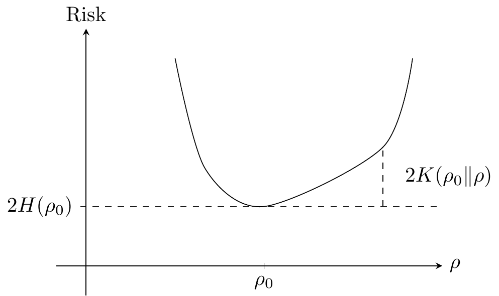
From the definition of the Kullback-Leibler divergence we have that for the negative log-likelihood loss, \[ \mathrm{Risk}(\rho) = 2H(\rho_0, \rho) = 2K(\rho_0\|\rho) + 2H(\rho_0). \tag{9.6}\] This decomposition has a similar interpretation as the bias-variance decomposition for the mean squared error. The entropy term corresponds to the variance term while the Kullback-Leibler term corresponds to the squared bias term. Minimizing the risk is equivalent to minimizing the Kullback-Leibler divergence.

As a direct consequence of Lemma 9.1 we see that the Kullback-Leibler divergence takes values in \([0,\infty)\) and equals \(0\) if and only if \(\rho = \rho_0\). It also follows directly from its integral representation above that its value does not depend upon the reference measure \(\nu\). The arbitrariness in the risk as well as the entropy cancels out in the Kullback-Leibler divergence. The Kullback-Leibler divergence can be interpreted as a distance from \(\rho_0\) to \(\rho\), but it is not a metric since it is neither symmetric nor does it fulfill the triangle inequality.

Example 9.2 If \(\rho = \mathcal{N}(\mu, \sigma^2)\) then \(\rho\) has a density w.r.t. Lebesgue measure, which is proportional to \(e^{-(y-\mu)^2/(2\sigma^2)}\), hence \[ - 2 \log h_{\mu}(y) = \frac{1}{\sigma^2} (y - \mu)^2. \]

The reference measure is taken to be \[ \frac{1}{\sqrt{2 \pi} \sigma} \cdot m, \] and the example does therefore not cover the comparison of two normal distributions with different variances.

If \(Y \sim \mathcal{N}(\mu_0, \sigma^2)\) we find that \[ \mathrm{Risk}(\rho) = \frac{1}{\sigma^2} E (Y - \mu)^2 = \frac{\mathrm{MSE}(\mu)}{\sigma^2}. \] The entropy⁵ is seen to be \(H(\rho_0) = 1/2.\) The Kullback-Leibler divergence of \(\rho\) from \(\rho_0\) is therefore \[ K(\rho_0\|\rho) = \frac{\mathrm{MSE}(\mu)}{2\sigma^2} - \frac{1}{2} = \frac{\mathrm{bias}^2(\mu)}{2\sigma^2}, \] which is precisely the squared bias relative to the variance as discussed in Example 9.1.

⁵ The entropy of the normal distribution is typically reported to be \[\log(\sigma \sqrt{2\pi e}) = \log(\sigma \sqrt{2\pi}) + \frac{1}{2},\] which is the differential entropy for which the reference measure is Lebesgue measure.

The example above shows the relation between the squared error loss and the negative log-likelihood loss for the normal distribution. For a semiparametric model of the mean – where a distributional assumption is not made – the squared error loss is still a sensible loss under a constant variance assumption.

Example 9.3 If \(\rho = \mathcal{E}(\theta, \nu_{\psi})\) is an exponential dispersion distribution then by (5.1) \[ - 2 \log h_{\theta}(y) = 2 \frac{\kappa(\theta) - \theta y}{\psi}, \] so if \(Y \sim \mathcal{E}(\theta_0, \nu_{\psi})\) the risk is given as \[ \mathrm{Risk}(\rho) = 2 \frac{\kappa(\theta) - \theta \mu(\theta_0)}{\psi}, \] where \(\mu\) is the mean value function.

The reference measure is taken as \(\nu_{\psi}\), and this example does therefore not cover the comparison of distributions with different dispersion parameters.

The entropy is similarly \[ H(\rho_0) = \frac{\kappa(\theta_0) - \theta_0 \mu(\theta_0)}{\psi}, \] and the Kullback-Leibler divergence is \[ \begin{align*} K(\rho_0\|\rho) & = \frac{(\mu(\theta_0)(\theta_0 - \theta) - \kappa(\theta_0) + \kappa(\theta))}{\psi} \\ & = \frac{d(\mu(\theta_0), \mu(\theta))}{2\psi} \end{align*} \] with \(d\) the unit deviance.

Note that in the example above the deviance \(d(y, \mu(\theta))\) is equal to \(-2 \log h_{\theta}(y)\) up to an additive constant that does not depend upon \(\theta\). We can therefore just as well replace the negative log-likelihood loss by the deviance in the computation of the risk. For comparison purposes, the constant will cancel out.

For any given unit deviance \(d\) the deviance loss, \(d(Y, \mu)\), can be computed for any probability distribution \(\rho\) on \(\mathbb{R}\), provided it has finite mean \[\mu = \int y \rho(\mathrm{d}y).\] Since the deviance loss depends only on the mean, it is useful for semiparametric models just as the squared error loss is, and it may be more appropriate than the squared error loss if the variance depends on the mean.

If \(\mathcal{V}\) denotes a variance function, an alternative semiparametric loss function is the Pearson loss \[ \frac{(Y - \mu)^2}{\mathcal{V}(\mu)}. \] For a mean-variance relation that does not correspond to an exponential dispersion model, the Pearson loss can always be used.

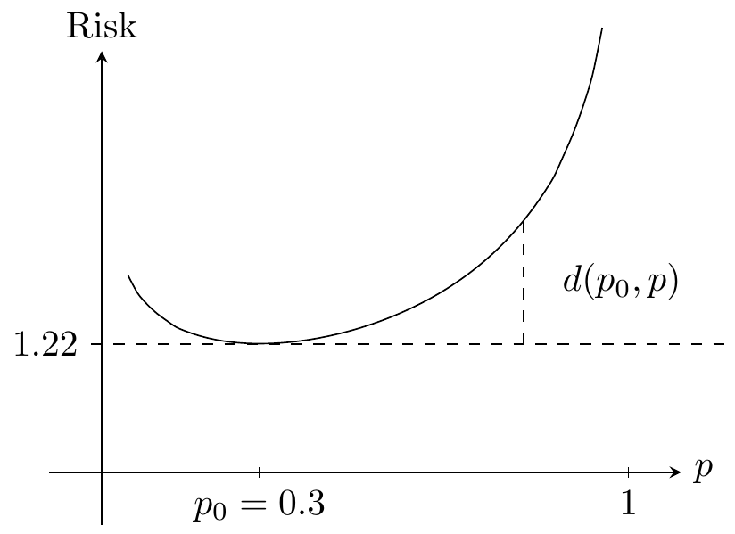
Example 9.4 From Example 5.10 it follows that the deviance for the Bernoulli distribution is \[ d(y, p) = 2y \log \Big(\frac{y}{p}\Big) + 2(1-y) \log \Big(\frac{1-y}{1-p}\Big) \] for \(y \in [0, 1]\) and \(p \in (0,1)\).

Though a Bernoulli variable will only take the values \(0\) or \(1\), the deviance is defined for \(y\) in the closed interval \([0,1]\).

If \(P(Y = 1) = p_0\) we get that \[ \mathrm{Risk}(p) = - 2 p_0 \log p - 2 (1-p_0) \log (1-p). \] The entropy is \[ H(p_0) = p_0 \log p_0 + (1-p_0) \log (1-p_0), \] and the Kullback-Leibler divergence is given by \[ \begin{align*} 2K(p_0\|p) & = \mathrm{Risk}(p) - 2 H(p_0) \\ & = 2 p_0 \log \Big(\frac{p_0}{p}\Big) + 2 (1-p_0) \log \Big(\frac{1-p_0}{1-p}\Big) \\ & = d(p_0, p). \end{align*} \]

Figure 9.6: Risk for the Bernoulli deviance is a convex function of the probability parameter \(p\). The true probability is \(p_0 = 0.3\) with entropy \(1.22 / 2 = 0.61\). The deviance \(d(p_0, p)\) equals twice the Kullback-Leibler divergence of \(p\) from \(p_0\).

9.3.2 Regression risk

For a regression model of \(Y\) conditionally on the predictor variable \(X\) there are two different ways of assessing the predictive strength of the model. Either conditionally on \(X = x\) or integrated over the distribution of \(X\). With \(\rho(x)\) denoting the probability model of \(Y\) given \(X = x\) it is thus possible to consider the conditional risk

The convention is that an expectation is always over all random variables inside the parentheses. That is, it is an integration out over the joint distribution of all variables. Conditional expectations are used when one or more variables are held fixed.

\[ \mathrm{Risk}(\rho(x)) = E \big( \mathrm{Loss}(Y, \rho(x)) \bigm| X = x\big), \] as well as the unconditional risk \[ \mathrm{Risk}(\rho) = E \big( \mathrm{Loss}(Y, \rho(X))) = E \big( \mathrm{Risk}(\rho(X)) \big), \] where the tower property of conditional expectations is used to get the last identity. The unconditional risk is also called the generalization error of the model \(\rho\). We denote it \(\mathrm{Risk}(\rho)\), but remember that \(\rho\) is now a map, \(x \mapsto \rho(x)\), that gives a model of the conditional distribution of \(Y\) given \(X = x\).

With \(m\) predictors \(X_1, \ldots, X_m\) and the conditional risk for the \(i\)-th response denoted \(\mathrm{Risk}_i(\rho(X_i))\), we can summarize the conditional risks as the average risk \[ \mathrm{Risk}_{\mathrm{avg}}(\rho) = \frac{1}{m} \sum_{i=1}^m \mathrm{Risk}_i(\rho(X_i)). \] When the empirical distribution of the observed predictors resembles the marginal distribution⁶ of \(X\), the average risk is a sensible estimate of \(\mathrm{Risk}(\rho)\). However, if the empirical distribution of the \(X_i\)-s does not match the distribution of \(X\), \(\mathrm{Risk}_{\mathrm{avg}}(\rho)\) can be a biased estimate of the unconditional risk. This is particularly problematic if the \(X_i\)-s are selected to overrepresent situations where the model gives very good predictions – whether or not the selection was deliberate to give a favorable validation or just due to ignorance.

⁶ Which is the case if \(X_1, \ldots, X_m\) are i.i.d. observations with the same distribution as \(X\) by the law of large numbers.

9.4 Error estimates

Practical model assessment requires that we can compute the generalization error \(\mathrm{Risk}(\hat{\rho})\) for the model, \(\hat{\rho}\), that has been fitted to data. Since \(\rho_0\) is unknown the theoretical formulas in the preceding section are of little value. The generalization error has to be estimated somehow. This section deals with the estimation of the generalization error.

Risk estimation is not straightforward because the data is already used once for fitting the model. If \(\hat{\rho}\) denotes the fitted model based on the data \((X_1, Y_1), \ldots, (X_n, Y_n)\), its average loss on the dataset is \[ \mathrm{err} = \frac{1}{n} \sum_{i=1}^n \mathrm{Loss}(Y_i, \hat{\rho}(X_i)). \tag{9.7}\] This number is also known as the training error. It is not a good estimate of neither the average risk nor the generalization error of \(\hat{\rho}\) because \((Y_i, X_i)\) and \(\hat{\rho}\) are dependent. It will typically have a downward bias, that is, it underestimates the generalization error and is thus too optimistic about the predictive strength of the model. As a rule of thumb, the more complex and flexible the model is, the more will \(\mathrm{err}\) underestimate the generalization error of \(\hat{\rho}\).

For the squared error loss \[ \mathrm{err} = \frac{\mathrm{RSS}}{n}, \] for the deviance loss \[ \mathrm{err} = \frac{D}{n}, \] where \(D\) is the total deviance and for the Pearson loss \[ \mathrm{err} = \frac{\chi^2}{n}, \] where \(\chi^2\) is the \(\chi^2\)-statistic.

It is possible that a complex model with a small training error is both a better fit to data and a better predictive model than a simple model. But it is also possible that the complex model overfits the data and is worse as a predictive model. For the linear model used in the bike rent example, the inclusion of a more flexible nonlinear expansion of a predictor variable appears to improve the model fit – up to some point – but eventually the model appears to pick up specific fluctuations in the data.

An overfitted model captures properties of the data that are specific to the given dataset, and which do not generalize to other data. An overfitted model may appear to fit the data very well, but it will have less predictive strength than a model that is not overfitted. For a given dataset there is always a limit to how complex a model we can fit without overfitting. The main challenge when assessing a model is to estimate its predictive strength correctly so that overfitted models are adjusted for their optimism.

9.4.1 Error estimation via validation data

To obtain an unbiased estimate of the risk of \(\hat{\rho}\) an independent validation dataset is required. That is, in addition to the data used for fitting \(\hat{\rho}\) we need an independent dataset \[(X_1^{\mathrm{new}}, Y_1^{\mathrm{new}}), \ldots, (X_m^{\mathrm{new}}, Y_m^{\mathrm{new}})\] with the \(Y_i^{\mathrm{new}}\)-s conditionally independent given the predictors and with \(Y_i^{\mathrm{new}}\) having conditional distribution \(\rho_0(X_i^{\mathrm{new}})\). In this case we define the estimator \[ \widehat{\mathrm{Risk}} = \frac{1}{m} \sum_{i=1}^m \mathrm{Loss}( Y_i^{\mathrm{new}}, \hat{\rho}(X_i^{\mathrm{new}})). \] It follows by the independence between \(\hat{\rho}\) and the validation data that \(\widehat{\mathrm{Risk}}\) is an unbiased estimate of the average risk, in the sense that \[ \begin{align*} E(\widehat{\mathrm{Risk}} \mid \hat{\rho}, \mathbf{X}^{\mathrm{new}}) & = \frac{1}{m} \sum_{i=1}^m E(\mathrm{Loss}( Y_i^{\mathrm{new}}, \hat{\rho}(X_i^{\mathrm{new}})) \mid \hat{\rho}, X_i^{\mathrm{new}})\\ & = \frac{1}{m} \sum_{i=1}^m \mathrm{Risk}_i(\hat{\rho}(X_i^{\mathrm{new}}))\\ & = \mathrm{Risk}_{\mathrm{avg}}(\hat{\rho}). \end{align*} \] Whether \(\widehat{\mathrm{Risk}}\) can be regarded as an unbiased estimate of the generalization error depends – as in the discussion above – on whether the empirical distribution of \(X_1^{\mathrm{new}}, \ldots, X_m^{\mathrm{new}}\) is representative of the distribution of future \(X\)-s.

Error estimation using validation data is fairly straightforward. It is, however, important not to make the mistake of peeping at the validation data while estimating \(\rho\). We should, for example, avoid preprocessing steps, such as data standardization, that use the validation data. While the inclusion of the validation data for standardization is a small blunder, it is a major mistake to include the validation data in a preprocessing variable selection step, say.

In practice, the validation dataset is obtained by setting aside a randomly selected subset containing 10-25% of the data available. The remaining 75-90% of the data is used for model fitting. If the dataset is small, setting aside a part of the data to be used for model assessment only is not a viable option. And we can in all cases argue that we could fit a better model if we used all data for the model fitting. The following section treats data splitting techniques that allow us to use all data for model fitting while still giving good estimates of predictive strength – with some extra computational costs.

What we call “validation data” is also known as “test data”. Sometimes, data is split in three parts with “training data” used to fit models, “test data” used to select among models and “validation data” used to assess the selected model.

9.4.2 Error estimation via data splitting

Data splitting techniques comprise a collection of procedures that mimic setting aside a validation dataset while not actually doing so. Hence the full dataset is used for fitting the model while the model assessment is based on the data splitting procedure. The data splitting procedures discussed in this section are all base on Assumption A6, that is, we assume that the observations \((X_1, Y_1), \ldots, (X_n, Y_n)\) are i.i.d.

Expected generalization error

A slightly tricky aspect of using data splitting techniques is that we will not directly estimate the generalization error of the model \(\hat{\rho}\) that is fitted to the entire dataset. We will instead estimate the expected generalization error.

Definition 9.3 With \((Y^{\mathrm{new}}, X^{\mathrm{new}})\) independent of \(\hat{\rho}\) the expected generalization error is defined as \[ \mathrm{Err} = E \big(\mathrm{Loss}(Y^{\mathrm{new}}, \hat{\rho}(X^{\mathrm{new}}))\big). \]

Observe that \(\hat{\rho}\) is random as a function of the data, thus by convention the expectation defining the generalization error is an expectation over the data as well.

It follows from the definition of the generalization error and the tower property of conditional expectations that \[ \mathrm{Err} = E\Big( E \big(\mathrm{Loss}(Y^{\mathrm{new}}, \hat{\rho}(X^{\mathrm{new}})) \bigm| \hat{\rho} \big) \Big) = E \big( \mathrm{Risk}(\hat{\rho}) \big). \] The hierarchy of error measures and estimates can be quite mind-boggling, but think about \(\mathrm{Err}\) as an assessment of the estimation method used for computing \(\hat{\rho}\) rather than an assessment of \(\hat{\rho}\) per se.

Example 9.5 (Squared error loss) For the squared error loss and any estimator \(\hat{m}\) of the regression function, we first condition on \(X^{\mathrm{new}} = x\). Then with \[ \begin{align*} m(x) & \coloneqq E(\hat{m}(x)) \\ m_0(x) & \coloneqq E(Y^{\mathrm{new}} \mid X^{\mathrm{new}} = x) \\ \sigma^2(x) & \coloneqq V(Y^{\mathrm{new}} \mid X^{\mathrm{new}} = x) \end{align*} \] we have \[ \mathrm{Risk}(\hat{m}(x)) = \mathrm{MSE}(\hat{m}(x)) = (m_0(x) - \hat{m}(x))^2 + \sigma^2(x), \] and we get the decomposition \[ \begin{align*} E( \mathrm{MSE}(\hat{m}(x)) ) & = E((m_0(x) - \hat{m}(x))^2) + \sigma^2(x) \\ & = (m_0(x) - m(x))^2 + E((m(x) - \hat{m}(x))^2) \\ & \quad + 2 (\mu_0(x) - m(x)) E(m(x) - \hat{m}(x))+ \sigma^2(x) \\ & = (m_0(x) - m(x))^2 + V(\hat{m}(x)) + \sigma^2(x) \\ & = \mathrm{bias}(x)^2 + \mathrm{variance}(x) + \sigma^2(x). \end{align*} \] where we have used that \(E(m(x) - \hat{m}(x)) = 0\) for the third identity. From this it follows that \[ \mathrm{Err} = \mathrm{bias}^2 + \mathrm{variance} + \sigma^2 \tag{9.8}\] where \[ \begin{align*} \mathrm{bias}^2 & = E(\mathrm{bias}^2(X)) \\ \mathrm{variance} & = E(\mathrm{variance}(X)) \\ \sigma^2 & = E(\sigma^2(X)). \end{align*} \] Thus the expected generalization error decomposes into a sum of three non-negative terms. The term \(\sigma^2\) is called the irreducible error, sometimes also known as the Bayes risk. It does not depend on the model or the estimator and lower bounds the expected generalization error for all models and estimators. The two other terms are the expected variance and the expected squared bias of the estimator – the expectation being over the marginal distribution of the predictor \(X\).

The decomposition given by Equation 9.8 is conceptually useful. It provides some insights about what the expected generalization error measures, and it tells us that to minimize the expected generalization error we need to minimize both the squared bias and the variance of the model/estimator. We generally expect that the more complex a model is, the smaller is the bias, but the larger is the variance of the estimator. Thus there is a bias-variance tradeoff. In practice it can be difficult to directly estimate the two terms \(\mathrm{bias}^2\) and \(\mathrm{variance}\), and the decomposition is therefore less useful for estimating the expected generalization error.

Data splitting procedures

To estimate \(\mathrm{Err}\) we turn to data splitting. Besides leading to estimators of the expected generalization error, these procedures also work for any choice of loss function – not just the squared error loss, say.

The three main data splitting procedures we describe below work by the same general principle. They consist of \(B\) rounds of data splitting, and in each round one subset of the dataset is used for fitting the model and the other works as an independent validation dataset. In round \(b\) for \(b = 1,\ldots, B\) the index set \(\{1, \ldots, n\}\) is divided into two disjoint subsets \(I(b)\) and \(J(b)\) followed by two steps:

1. The model \(\hat{\rho}_b\) is fitted based on data with indices in \(I(b)\).
2. The losses \(\mathrm{L}(b,i) = \mathrm{Loss}(Y_i, \hat{\rho}_b(X_i))\) are computed for \(i \in J(b)\).

After the \(B\) rounds of model fitting and loss computation the average loss is computed as \[ \widehat{\mathrm{Err}} = \frac{1}{N} \sum_{b=1}^B \sum_{i \in J(b)} \mathrm{L}(b,i) \tag{9.9}\] with \(N = \sum_{b=1}^B |J(b)|\). It is essential that the model \(\hat{\rho}_b\) is fitted to the data given by the index set \(I(b)\) in exactly the same way as \(\hat{\rho}\) is fitted to the full dataset. This includes any kind of variable selection, parameter tuning or the like that might be carried out as part of the model fitting. Otherwise \(\widehat{\mathrm{Err}}\) could be overly optimistic.

A complete specification of a data splitting procedure requires that the division of the index set is specified. The following three are the most used:

Subsampling: Subset \(I\) of size \(m < n\) is sampled without replacement from \(\{1, \ldots, n\}\) and \(J\) is the complement of \(I\).

Cross-validation (\(K\)-fold): The index set \(\{1, \ldots, n\}\) is randomly divided into \(K\) disjoint sets \(H_1, \ldots, H_K\) of roughly equal size \(\approx n/K\). This defines \(K\) rounds of data splitting with \(I(k) = \{1, \ldots, n\} \backslash H_k\) and \(J(k) = H_k\) for \(k = 1, \ldots, K\).

For cross-validation, \(B = MK\) is always an integer multiple \(M \in \mathbb{N}\) of \(K\).

Bootstrapping: Subset \(I\) of size \(n\) (replicates counted with multiplicities) is sampled with replacement from \(\{1, \ldots, n\}\) and \(J\) is the complement of \(I\).

Remember that the estimate \(\hat{\rho}\) is computed using all \(n\) observations in the dataset, but that the data splitting procedures result in an average of losses computed for different estimates based on different subsets of the full dataset. We can therefore not regard \(\widehat{\mathrm{Err}}\) as an estimate of the generalization error⁷ \(\mathrm{Risk}(\hat{\rho})\). It is, however, fairly clear that the data splitting procedures are empirically mimicking the definition of the expected generalization error \(\mathrm{Err}\): the model is fitted on one part of the data and the loss is computed on an independent part, and the losses are the averaged. Intuitively, \(\widehat{\mathrm{Err}}\) is therefore an estimate of \(\mathrm{Err}\).

⁷ To estimate \(\mathrm{Risk}(\hat{\rho})\) we really need an independent validation dataset.

Since \(\mathrm{Err}\) is a quantification of the estimation procedure rather than the specific estimate \(\hat{\rho}\), it is essential that the entire model fitting process is properly accounted for. To avoid overly optimistic error estimates, the estimation procedure should preferable be completely specified prior to seeing data, and \(\hat{\rho}\) should then be computed according to that procedure. The estimates computed in the data splitting process can then be computed in exactly the same way. This can be difficult to do in practice, since elements of human judgement, such as studying residual plots, are often part of the model fitting process in real world applications.

An important step towards more valid error estimates is to represent the entire model fitting process programmatically to the greatest extent possible⁸. This is one very good reason for documenting your data analysis in R scripts or Quarto documents and for wrapping up entire methods as new R functions instead of working interactively.

⁸ Hardliners would accept only programmatic model fitting procedures. This goes against seeing data analysis as a fundamentally interactive discipline. Both viewpoints have merits, and the concrete application should determine which considerations are given the biggest weight. It requires human judgement!

Example 9.6 (Bike rental revisited) We return to the bike rental example and implement \(K\)-fold cross-validation for the squared error loss and for linear models that can be specified via a formula.

cv <- function(form, data, K = 10, M = 20) {
    n <- nrow(data)
    response <- all.vars(form)[1]
    loss <- vector("list", M)
    mu_hat <- numeric(n)
    for(b in 1:M) {
        # Generating the random subdivision into groups
        group <- sample(rep(1:K, length.out = n))
        for(i in 1:K) {
            model <- lm(form, data = data[group != i, ])
            mu_hat[group == i] <- predict(model, newdata = data[group == i, ])
        }
    loss[[b]] <- (data[, response] - mu_hat)^2
    }
    unlist(loss) |> mean()
}

We then run cross-validation for the sequence of models with \(\mathrm{df}\) ranging from \(1\) to \(12\), and we also compute the training MSE. We use the default settings with \(K = 10\) and \(M = 20\) in the implementation of cv() above. That is, we do \(10\)-fold cross-validation for \(20 \cdot 10 = 200\) rounds.

set.seed(42)
cv_bike <- tibble(
    df = 1:12,
    cv = Vectorize(\(d) cv(Count ~ ns(Temperature, df = df[d]), bike))(df),
    mse = Vectorize(\(d) lm(Count ~ ns(Temperature, df = df[d]), bike) |> 
        (\(x) residuals(x)^2)() |> mean())(df)
)

Figure 9.7: Training MSE (red) and cross-validated MSE (blue).

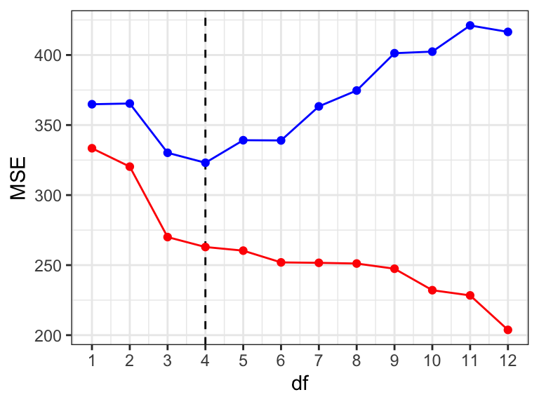
Figure 9.7 shows the resulting training MSE and cross-validated MSE. We make the following three observations:

1. The traning MSE (red) is monotonely decreasing with model complexity. This is in accordance with our previous observations.
2. The cross-validated MSE (blue) is always larger than the training MSE. This is expected and reflects the optimism of the training error. We note that this optimism increases with model complexity.
3. The cross-validated MSE (blue) attains a minimum for \(\mathrm{df} = 4\). This shows that the model with optimal (expected) predictive performance is the model with \(\mathrm{df} = 4\).

Properties of data splitting estimators

A formal justification that \(\widehat{\mathrm{Err}}\) is actually a good estimate of the expected generalization error is a bit involved, and we will only give some superficial arguments.

We should first observe that \(\mathrm{Err}\) actually depends on the size of the dataset \(n\) used for fitting the model. To emphasize this dependence we write \(\mathrm{Err}(n)\) whenever needed. The graph of \(\mathrm{Err}(n)\) as a function of \(n\) is known as the error curve⁹. It will typically be monotonely decreasing and bounded below. If the sets \(I(b)\) in the data splitting procedure are all of roughly equal size, \(|I(b)| \approx m\) for all \(b\), say, it is appropriate¹⁰ to regard \(\widehat{\mathrm{Err}}\) as an estimate of \(\mathrm{Err}(m)\) rather than \(\mathrm{Err}(n)\). If \(m < n\) and the error curve is steep around \(m\), \(\widehat{\mathrm{Err}}\) will overestimate \(\mathrm{Err}(n)\).

⁹ A close relative to the learning curve, which is given by \(c - \mathrm{Err}(n)\) for some suitable constant \(c\).

¹⁰ For subsampling and cross-validation but not bootstrapping.

For subsampling it follows directly that \[ E\big(\widehat{\mathrm{Err}}\big) = \mathrm{Err}(m) \qquad \text{(subsampling)} \] and for \(K\)-fold cross-validation \[ E \big(\widehat{\mathrm{Err}}\big) \approx \mathrm{Err}((1 - 1/K) n) \qquad \text{(cross-validation).} \] For small datasets the error curve may be rather steep in a neighborhood of \(n\), and it is recommended to take \(K = 10\) to obtain an estimate of \(\mathrm{Err}(0.9 n)\). For large datasets the error curve may be less steep and taking \(K = 5\) to obtain an estimate of \(\mathrm{Err}(0.8 n)\) will suffice.

The situation for bootstrapping is more complicated. Even though \(|I(b)| = n\), some of the data points appear multiple times due to the sampling with replacement. Efron (1983) showed that \(E \big(\widehat{\mathrm{Err}}\big)\) agrees with \(\mathrm{Err}(n/2)\) up to second order, which makes the bootstrap method comparable with \(2\)-fold cross-validation. This gives a potential bias of the method. Several corrections exist but they will not be pursued here, see Efron and Tibshirani (1997).

Efron, Bradley. 1983. “Estimating the Error Rate of a Prediction Rule: Improvement on Cross-Validation.” Journal of the American Statistical Association 78 (382): 316–31.

Efron, Bradley, and Robert Tibshirani. 1997. “Improvements on Cross-Validation: The 632+ Bootstrap Method.” Journal of the American Statistical Association 92 (438): 548–60.

There is some instability of \(\widehat{\mathrm{Err}}\) caused by the random splitting. This can be reduced by replicating the data splitting procedure to give as many rounds as is computationally feasible. For \(K\)-fold cross-validation the number of rounds are integer multiples \(M\) of \(K\). Cross-validation can sensibly be used with \(M = 1\) giving the minimal number of \(K\) rounds, which makes it only moderately computationally demanding. Among the three data splitting procedures, cross-validation with \(K = 5\) or \(K=10\) is the most widely used and recommended as it usually strikes a good balance between computation time and stability of \(\widehat{\mathrm{Err}}.\) Adding extra rounds will increase the stability of the estimate \(\widehat{\mathrm{Err}}\) but also increase the computational burden. Acceptable stability of \(\widehat{\mathrm{Err}}\) usually requires more than 5–10 rounds for subsampling or bootstrapping.

The special case of \(n\)-fold cross-validation is also known as leave-one-out cross-validation. There is no instability in this procedure, just \(n\) rounds of model fitting to \(n-1\) data points and loss computation for the last omitted data point. The computation time scales in principle linearly with the size of the dataset, which makes it computationally intractable for large datasets. However, for a class of estimators that are linear in the response there exists an analytic shortcut, which allows for the computation of leave-one-out estimate of \(\widehat{\mathrm{Err}}\) directly from the original model fit. In this case leave-one-out cross-validation can be a computationally cheap alternative to the other data splitting procedures.

Irrespectively of the data splitting procedure used, it is difficult to quantify the uncertainty of \(\widehat{\mathrm{Err}}\) as an estimator of \(\mathrm{Err}\). The estimator is an average of dependent variables and we cannot easily estimate its variance, say. It is common for cross-validation with \(B = K\) (that is, \(M = 1\)) to pretend that the terms in (9.9) are i.i.d. and compute standard errors under this assumption. This is an acceptable heuristic, but generally we don’t have any good finite sample approximations of the distribution of \(\widehat{\mathrm{Err}}\). The distributions of the different error estimators are explored empirically in a simulation study in Section 9.5.

9.4.3 Analytic error estimates

In the previous section the training error, \(\mathrm{err}\), was discarded as a valid error estimate. Alternatives were described based on the idea of using independent validation data for error estimation. This section gives analytic error estimates that can be understood as bias corrections of \(\mathrm{err}\). These analytic estimates do not rely on independent validation or repeated data splitting and refitting of the model, and they can typically be computed efficiently. This comes at the price of added model assumptions, and the analytic error estimates are unfortunately estimates of yet another error quantity closely related to – but not exactly the same as – the average risk.

Definition 9.4 With \(Y_1^{\mathrm{new}}, \ldots, Y_n^{\mathrm{new}}\) conditionally independent of \(\hat{\rho}\) given \(\mathbf{X}\) and with the same conditional distribution as \(Y_1, \ldots, Y_n\) the in-sample error is defined as \[ \mathrm{Err}_{\mathrm{in}} = \frac{1}{n} \sum_{i=1}^n E \big(\mathrm{Loss}(Y_i^{\mathrm{new}}, \hat{\rho}(X_i)) \mid \mathbf{X}\big). \]

Observe that \(E(\mathrm{Err}_{\mathrm{in}})\) is not equal to \(\mathrm{Err}\) in general. There is a difference between reusing the \(X_i\)-s or using independent \(X_i^{\mathrm{new}}\)-s for the prediction.

The general definition above of the in-sample error is based on Assumption A5 of conditionally independence of the response variables given the predictors, which is weaker than Assumption A6. This is sensible as the in-sample error fixes the predictors to be the observed predictions, and it is therefore also a weaker quantification of predictive stength than the (expected) generalization error. It can, nevertheless, still be useful for model comparisons.

The main reason we consider the in-sample error is that we can derive analytic representations of it that links it to the training error, and which can be used for easy estimation without using independent validation data or data splitting. For the deviance loss the following theorem gives such a representation of the in-sample error where any reference to independent data is eliminated.

Theorem 9.1 If the loss is the unit deviance for an exponential dispersion model with corresponding canonical link function \(g\) then \[ \mathrm{Err}_{\mathrm{in}} = E (\mathrm{err} \mid \mathbf{X}) + \frac{2}{n} \sum_{i=1}^n \mathrm{cov}(g(\hat{\mu}_i), Y_i \mid \mathbf{X}). \tag{9.10}\]

Recall that for a generalized linear model, \[ \hat{\mu}_i = \mu(X_i^T\hat{\beta}), \] but Theorem 9.1 does actually not make any assumption on how \(\hat{\mu}_i\) is estimated.

Proof. From Definition 5.5 of the deviance, or rather Equation 5.4, \[ d_i^{\mathrm{new}} \coloneqq d(Y_i^{\mathrm{new}}, \hat{\mu}_i) = r(Y_i^{\mathrm{new}}) - 2 g(\hat{\mu}_i) Y_i^{\mathrm{new}} + 2 \kappa(g(\hat{\mu}_i)) \] and \[ d_i \coloneqq d(Y_i, \hat{\mu}_i) = r(Y_i) - 2 g(\hat{\mu}_i) Y_i + 2 \kappa(g(\hat{\mu}_i)) \] for some function \(r\). Subtracting these two quantities and taking conditional expectation given \(\mathbf{X}\) yields \[ E(d_i^{\mathrm{new}} - d_i \mid \mathbf{X}) = 2 E(g(\hat{\mu}_i)(Y_i - Y_i^{\mathrm{new}}) \mid \mathbf{X}) \] since \(Y_i\) and \(Y_i^{\mathrm{new}}\) are assumed to have the same conditional distribution. This implies, additional, that \(Y_i - Y_i^{\mathrm{new}}\) has conditional mean \(0\), and the right hand side above is a covariance. Thus \[ \begin{align*} E(d_i^{\mathrm{new}} - d_i \mid \mathbf{X}) & = 2 \mathrm{cov}(g(\hat{\mu}_i), Y_i - Y_i^{\mathrm{new}} \mid \mathbf{X}) \\ & = 2 \mathrm{cov}(g(\hat{\mu}_i), Y_i \mid \mathbf{X}) \end{align*} \] since \(Y_i^{\mathrm{new}}\) is conditionally independent of \(\hat{\mu}_i\). This gives that \[ \begin{align*} \mathrm{Err}_{\mathrm{in}} & = \frac{1}{n} \sum_{i=1}^n E (d_i^{\mathrm{new}} \mid \mathbf{X}) \\ & = \frac{1}{n} \sum_{i=1}^n E (d_i \mid \mathbf{X} ) + \frac{1}{n} \sum_{i=1}^n 2 \mathrm{cov}(g(\hat{\mu}_i), Y_i \mid \mathbf{X}) \\ & = E(\mathrm{err} \mid \mathbf{X}) + \frac{2}{n} \sum_{i=1}^n \mathrm{cov}(g(\hat{\mu}_i), Y_i \mid \mathbf{X}). \end{align*} \]

The proof is base on the deviance formula in Equation 5.4, which always holds for \(Y_i \in J\), but was shown to hold also for \(Y_i \in \overline{J} \backslash J\) for some specific cases, including the binomial and Poisson models.

Equation 9.10 may appear intimidating at first, but it is really quite interpretable. Clearly, \(\mathrm{err}\) is an unbiased estimate of \(E(\mathrm{err} \mid \mathbf{X})\), but (9.10) shows that it is biased as an estimate of the in-sample error. The bias is expressed in terms of the covariances between \(g(\hat{\mu}_i)\) and \(Y_i\), which makes good sense. A large positive correlation between the response \(Y_i\) and the value \(g(\hat{\mu}_i)\) for \(i = 1, \ldots, n\) indicates that the \(\hat{\mu}_i\)-s will be somewhat worse at predicting independent \(Y_i^{\mathrm{new}}\)-s than \(\mathrm{err}\) suggests.

Definition 9.5 For a canonical link function \(g\) the corresponding effective degrees of freedom of the estimator \(\hat{\mu}_i\), \(i = 1, \ldots, n\), is defined as \[ \mathrm{df} = \frac{1}{\psi} \sum_{i=1}^n \mathrm{cov}(g(\hat{\mu}_i), Y_i \mid \mathbf{X}). \]

The effective degrees of freedom only makes sense when using the deviance corresponding to the canonical link \(g\) as loss. However, it makes sense for any choice of estimator \(\hat{\mu}_i\).

If \(\hat{\mathrm{df}}\) denotes a suitable estimator of the effective degrees of freedom we can estimate the in-sample error as \[ \widehat{\mathrm{Err}}_{\mathrm{in}} = \mathrm{err} + 2 \frac{\hat{\psi}}{n} \hat{\mathrm{df}}, \tag{9.11}\] where \(\hat{\psi}\) denotes an estimator of the dispersion parameter (if it needs to be estimated). For a generalized linear model we can use the estimator
\[ \hat{\psi} = \frac{1}{n-p} \mathcal{X}^2 \] of the dispersion parameter, where \(\mathcal{X}^2\) is the Pearson \(\mathcal{X}^2\)-statistic for the model with \(p\) parameters. If \(\widehat{\mathrm{Err}}_{\mathrm{in}}\) is used for comparing multiple models, we should use a single model with a small bias (large \(p\)) to estimate \(\psi\). A closely related quantity is Mallows’s \(C_p\)-statistic, which is defined as \[ C_p = n \, \widehat{\mathrm{Err}}_{\mathrm{in}} = n \, \mathrm{err} + 2 \hat{\psi} \ \hat{\mathrm{df}}. \] From a predictive point of view it is sensible to use \(\widehat{\mathrm{Err}}_{\mathrm{in}}\) or \(C_p\) for comparison of two models whether they are nested or not. The smaller \(\widehat{\mathrm{Err}}_{\mathrm{in}}\) is the better is the model.

For (9.11) to be of practical use we need to be able to compute or estimate the effective degrees of freedom. The following examples show that it is, indeed, possible to compute this number in several different situations.

Example 9.7 (Squared error loss and linear estimators) Suppose that \(\hat{\mu}_i = (\mathbf{S} \mathbf{Y})_i\) for an \(n \times n\) matrix \(\mathbf{S}\) (which depends on \(\mathbf{X}\) but not \(\mathbf{Y}\)). Such an estimator is called linear. The projection estimator derived in Section 2.5 for the linear model is a linear estimator given by \[ \mathbf{S} = \mathbf{X} (\mathbf{X}^T \mathbf{X})^{-1} \mathbf{X}^T. \]

Many so-called smoothers are, in fact, linear estimators for a suitable choice of matrix \(\mathbf{S}\) – hence the notation \(\mathbf{S}\) for smoother.

Suppose also that the distributional assumptions A2 and A4 are fulfilled¹¹. We can then observe that for the squared error loss with corresponding canonical link being the identity, the effective degrees of freedom equals \[ \begin{align*} \mathrm{df} & = \frac{1}{\sigma^2} \sum_{i=1}^n \mathrm{cov}(\hat{\mu}_i, Y_i \mid \mathbf{X}) \\ & = \frac{1}{\sigma^2} \sum_{i,j=1}^n \mathrm{cov}(S_{ij} Y_j, Y_i \mid \mathbf{X})\\ & = \frac{1}{\sigma^2} \sum_{i=1}^n S_{ii} \sigma^2 \\ & = \mathrm{trace}(\mathbf{S}). \end{align*} \] Thus \[ \mathrm{Err}_{\mathrm{in}} = E (\mathrm{err} \mid \mathbf{X}) + \frac{2 \sigma^2}{n} \mathrm{trace}(\mathbf{S}). \] and \[ \widehat{\mathrm{Err}}_{\mathrm{in}} = \mathrm{err} + \frac{2 \hat{\sigma}^2}{n} \mathrm{trace}(\mathbf{S}). \]

¹¹ Note that there is no assumption about the conditional expectation of the \(Y_i\)-s. It is only assumed that they are conditionally uncorrelated and have homogeneous variance.

When \(\mathbf{S}\) is an orthogonal projection its trace is equal to the dimension \(p\) of its image, in which case \[ \widehat{\mathrm{Err}}_{\mathrm{in}} = \mathrm{err} + \frac{2 \hat{\sigma}^2 p}{n}. \tag{9.12}\]

Example 9.8 (Bike rentals revisited) All the models considered for the bike rental example are linear models, and we can use (9.12) to estimate the in-sample error. Doing so, we also add cross-validation errors estimated using either \(5\)-fold or \(20\)-fold cross-validation – in addition to \(10\)-fold cross-validation already considered in Example 9.6.

n <- nrow(bike)
sigma_sq_hat <- cv_bike$mse[12] * n / (n - 13)
cv_bike <- mutate(
    cv_bike, 
    mse_in = mse + 2 * sigma_sq_hat * (df + 1) / n,
    cv_5 = Vectorize(\(d) cv(Count ~ ns(Temperature, df = df[d]), bike, K = 5))(df),
    cv_25 = Vectorize(\(d) cv(Count ~ ns(Temperature, df = df[d]), bike, K = 25))(df),
)

Figure 9.8: Training MSE (red), cross-validated MSE (purple: \(K = 5\); blue: \(K = 10\); light blue: \(K = 25\)) and in-sample MSE (orange). The horizontal dashed line is \(\hat{\sigma}^2\) (an estimate of the lower bound on MSE).

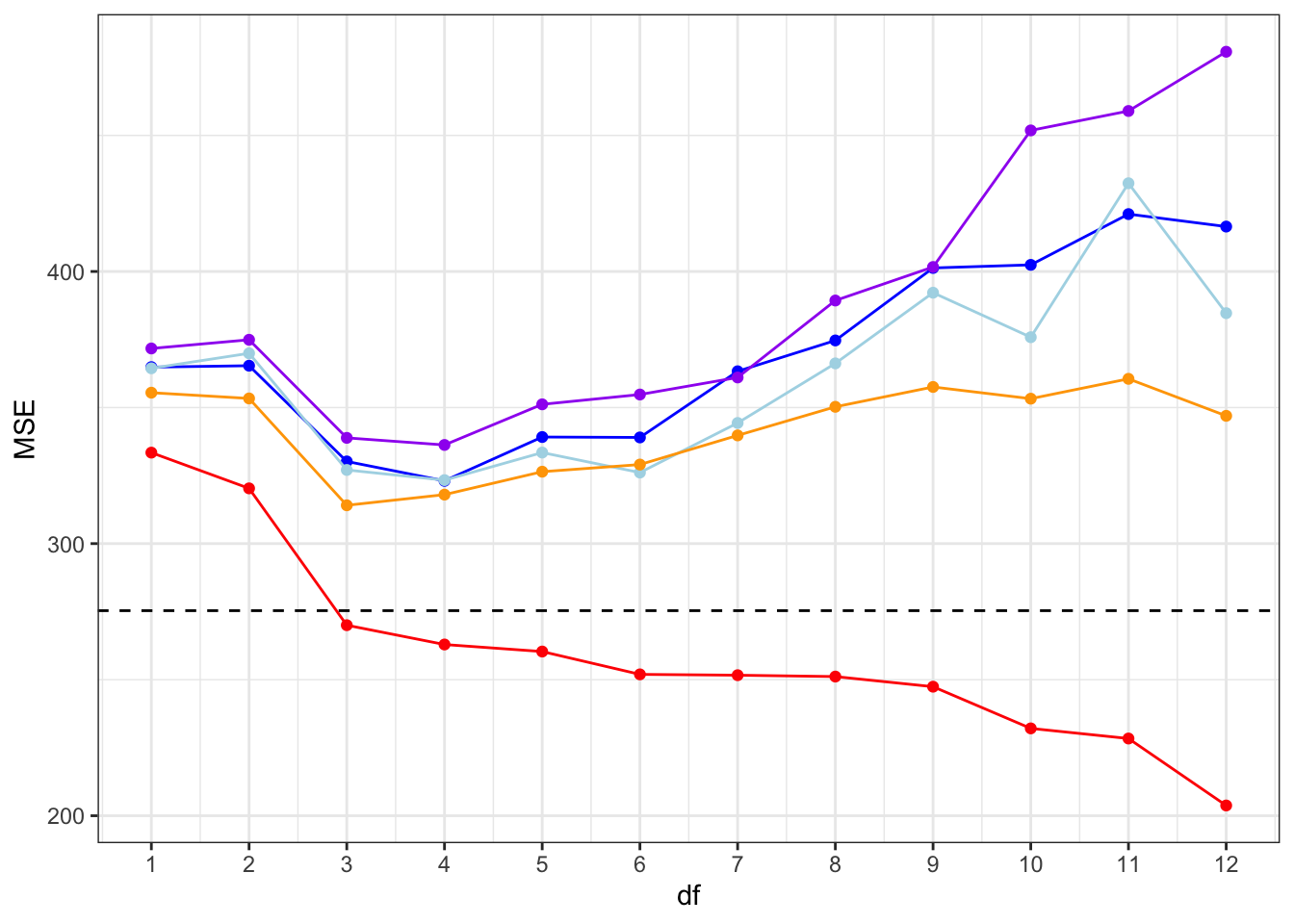
Figure 9.8 shows that even though there are differences both between the in-sample error and the cross-validated errors and within the cross-validated errors depending on the folds, all the error estimates have a similar shape and agree that models with \(\mathrm{df} = 3\) or \(\mathrm{df} = 4\) are best.

As discussed in Section 9.4, \(5\)-fold cross-validation is in this case effectively estimating \(\mathrm{Err}(40)\), corresponding to a sample size of \(n = 40\). Since \(10\)-fold and \(25\)-fold cross-validation correspond to estimating \(\mathrm{Err}(45)\) and \(\mathrm{Err}(48)\), respectively, and since we expect \(\mathrm{Err}(40) > \mathrm{Err}(45) > \mathrm{Err}(48) > \mathrm{Err}(50)\), the ordering of the cross-validated error estimates is unsurprising. We note that the in-sample error is generally smaller than the cross-validated errors, but it resembles \(25\)-fold cross-validation more than \(5\)-fold cross-validation.

It is possible to justify a generalization of Equation 9.11 to generalized linear models when the estimator is the MLE and the link function is canonical.

Example 9.9 Assume that \(\hat{\mu}_i = \mu(X^T_i \hat{\beta}^{\mathrm{ideal}})\) with \(\hat{\beta}^{\mathrm{ideal}}\) the idealized least squares estimator introduced in Section 6.3.1, and the \(\mu = g^{-1}\) is the inverse of the canonical link \(g\). Then \(g(\hat{\mu}_i) = (\mathbf{S} \mathbf{Z})_i\) for \[ \mathbf{S} = \mathbf{X} (\mathbf{X}^T \mathbf{W} \mathbf{X})^{-1} \mathbf{X}^T \mathbf{W}. \] Under the distributional assumptions GA2 and A4, \(Z_i\) is conditionally uncorrelated with \(Y_j\) for \(i \neq j\) and \[ \mathrm{cov}(Z_i, Y_i \mid \mathbf{X}) = \frac{\psi \mathcal{V}(\mu_i)}{\mu_i'} = \psi, \] since \(\mu = g^{-1}\). As in Example 9.7 we conclude that \[ \sum_{i=1}^n \mathrm{cov}(\hat{\mu}_i, Y_i \mid \mathbf{X}) = \psi \mathrm{trace}(\mathbf{S}). \] Now \[ \begin{align*} \mathrm{trace}(\mathbf{S}) & = \mathrm{trace}\Big(\mathbf{X} (\mathbf{X}^T \mathbf{W} \mathbf{X})^{-1} \mathbf{X}^T \mathbf{W}\Big) \\ & = \mathrm{trace}\Big((\mathbf{X}^T \mathbf{W} \mathbf{X})^{-1} \mathbf{X}^T \mathbf{W} \mathbf{X} \Big) \\ & = \mathrm{trace}(I_p) = p, \end{align*} \] where \(I_p\) denotes the \(p \times p\) identity matrix.

AIC

In addition to the estimate of the in-sample error or Mallows’s \(C_p\) above, AIC must be mentioned as another classical analytic way to quantify a model’s predictive stength. As stated below, AIC is up to scaling by the dispersion parameter identical to Mallows’s \(C_p\) if the deviance loss is used.

Definition 9.6 Assume that \(\rho_i = \rho_i(\beta)\) for \(\beta \in \mathbb{R}^p\) a \(p\)-dimensional parameter \(\beta\). With \(\ell\) the negative log-likelihood loss we define Akaike’s information criteria as \[ \mathrm{AIC} = 2 \sum_{i=1}^n \ell(\hat{\rho}_i) + 2 p. \]

The factor “2” in the definition of AIC is a somewhat arbitrary convention.

In the context of generalized linear models¹² we observe that \[ \mathrm{AIC} = \frac{1}{\psi} D + 2p \] where \(D = \sum_{i=1}^n d(Y_i, \hat{\mu}_i)\) is the deviance in Definition 6.2. The log-likelihood and hence AIC is only determined up to an additive constant. The estimator of \(\mathrm{Risk}\) derived from AIC is \[ \frac{1}{2n} \mathrm{AIC}. \]

¹² Either assuming that we know the dispersion parameter or that we just plainly ignore that it is estimated too. If it is estimated we should use a single value for all models as discussed above in relation to Mallows’s \(C_p\).

The justification of AIC hinges on a number of assumptions, and its justification is asymptotic for \(n \to \infty\). We will not pursue the arguments in any detail, but just mention three important assumptions for \(\mathrm{AIC}\) to be justifiable:

1. The estimator must be \(\hat{\rho}_i = \rho_i(\hat{\beta})\) with \(\hat{\beta}\) the maximum likelihood estimator.
2. The data generating model must be of the form \(\rho(\beta)\) for some \(\beta\), thus AIC is invalid if the model is misspecified.
3. For comparability of AIC between two models it is essential that the same reference measure is used for the definition of the likelihood.

One has to pay particular attention to point 3 above for generalized linear models. For example, the Poisson and the binomial distributions have different structure measures as exponential families¹³. If we do not account for this, the models are incomparable in terms of their AIC. This is unsurprising from a risk perspective as different models give different deviance loss functions. When comparing models we must use the same loss function throughout.

¹³ One has the factor \(\frac{1}{Y!}\) and the other \({m \choose Y}\) on the counting measure.

9.5 Data splitting estimators compared

This section illustrates aspects of the practical implementation of data splitting for quantification of predictive strength. This is done via a simulation study using the squared error loss, which also results in a comparison of the different data splitting procedures and the empirical distribution of their resulting estimators.

9.5.1 Implementations in R

We first implement a couple of general functions for computing training error, validation error and estimates of expected generalization error by subsampling or boostrapping. We have already implemented cross-validation in Section 9.4.2, which we reuse.

train_err <- function(form, data) { 
  model <- lm(form, data = data)
  residuals(model)^2 |> mean()
}

val_err <- function(form, data, newdata) { 
  response <- all.vars(form)[1]
  model <- lm(form, data = data)
  (newdata[, response] - predict(model, newdata = newdata))^2 |> unlist() |> mean()  
}

The two functions implemented below compute estimates of expected generalization error using subsampling and bootstrapping. Their implementations are quite similar and similar to the implementation of cv() in Example 9.6.

subsamp <- function(form, data, B = 200, q = 0.9) {
    n <- nrow(data)
    response <- all.vars(form)[1]
    loss <- vector("list", B)
    for(b in 1:B) {
        # Subsampling a data set of size q * n 
        i <- sample(n, floor(q * n))  
        model <- lm(form, data = data[i, ])
        mu_hat <- predict(model, newdata = data[- i, ])
        loss[[b]] <- (data[-i, response] - mu_hat)^2
    }
    unlist(loss) |> mean()
}

boot <- function(form, data, B = 200) {
    n <- nrow(data)
    response <- all.vars(form)[1]
    loss <- vector("list", B)
    for(b in 1:B) {
        i <- sample(n, n, replace = TRUE)
        model <- lm(form, data = data[i, ])
        mu_hat <- predict(model, newdata = data[- i, ])
        loss[[b]] <- (data[-i, response] - mu_hat)^2
    }
    unlist(loss) |> mean()
}

9.5.2 Simulation study

First we apply the different functions on a single data set for a simple linear regression model with \(p_0\) predictors. None of the predictors are related to the normally distributed response, whence we simulate from the model with \[ Y \mid X \sim \mathcal{N}(0, \sigma^2). \] In the simulations we fix \(p_0 = 20\) and \(\sigma^2 = 1\).

sim_yx <- function(n, p0) {
    x <- matrix(rnorm(p0 * n), n, p0)
    tibble(
        y = rnorm(n),
        as_tibble(x, .name_repair = "unique_quiet")
    )
}
n <- 100
p0 <- 20
# p = p0 + 1 = 21 as there will also be an intercept
set.seed(21)
yx <- sim_yx(n, p0)
form <- y ~ . # Includes all 20 variables as predictors

train	subsamp.	cv	bootstrap
0.73	1.24	1.21	1.47

Table 9.3: Four error estimates from running the simulation once.

Table 9.3 shows four error estimates for the single simulation above. With reference to Example 9.5 we know that the lower bound on the expected generalization error is \(\sigma^2 = 1\) (the Bayes risk). The training error in Table 9.3 is smaller, illustrating the optimism of the training error. The other three error estimates in Table 9.3 are larger, and the bootstrap estimate is notably larger than the two others.

In this example we can actually compute the expected training error¹⁴. Since \(\mathrm{err} = \hat{\sigma}^2 \frac{n - p}{n}\), it follows from Theorem 2.2 that \[ E(\mathrm{err}) = E(\mathrm{err} \mid \mathbf{X}) = \sigma^2(1 - \frac{p}{n}) = 1 - 21/100 = 0.79. \] The in-sample error can then also be computed as \[ \mathrm{Err}_{\mathrm{in}} = E(\mathrm{err} \mid \mathbf{X}) + 2 \frac{p}{n} = 1 + 21 / 100 = 1.21. \]

¹⁴ Unconditionally as well as conditionally on \(\mathbf{X}\).

For subsampling with \(q = 0.9\) and for \(10\)-fold cross-validation, the error estimates have mean \(\mathrm{Err}(90)\) and the bootstrapping error estimate has approximately mean \(\mathrm{Err}(50)\). Though these numbers are not exactly the same as the corresponding in-sample errors for \(n = 90\) and \(n = 50\), which are \(1.23\) and \(1.42\), respectively, they turn out to be relatively close.

In the simulation above a large number of rounds (\(B = 200\)) were used. In real applications this may be computationally prohibitive as this requires a large number of refits of the model. Below we investigate by simulations the distribution of the error estimators, and we study the effect of the number of rounds \(B\) on these distributions.

First we take \(B = 10\) rounds, which for \(10\)-fold cross-validation corresponds to a single outer loop (\(M = 1\)).

err_hat <- vector("list", 200)
for(m in seq_along(err_hat)) {
  yx <- sim_yx(n, p0)
  yx_new <- sim_yx(n, p0)
  err_hat[[m]] <- tibble(
    train = train_err(form, yx), 
    validation = val_err(form, yx, yx_new),
    subsamp. = subsamp(form, yx, B = 10),
    cv = cv(form, yx, K = 10, M = 1),
    bootstrap = boot(form, yx, B = 10)
  )
}

err_hat <- do.call(rbind, err_hat) |> 
    tidyr::pivot_longer(
        cols = everything(), 
        names_to = "Method", 
        values_to = "Squared error"
    ) |> 
    mutate(
        Method = factor(Method, c("train", "validation", "subsamp.", "cv", "bootstrap"))
    )

ggplot(err_hat, aes(x = Method, y = `Squared error`)) + 
  geom_violin(fill = gray(0.8)) + 
  geom_hline(yintercept = 1 + (p0 + 1) / n, color = "red", alpha = 0.5, linewidth = 1) +
  geom_hline(yintercept = 1 - (p0 + 1) / n, color = "blue", alpha = 0.5, linewidth = 1) +
  stat_summary(fun = mean, color = "blue", geom = "point") +
  coord_cartesian(ylim = c(0, 2.5))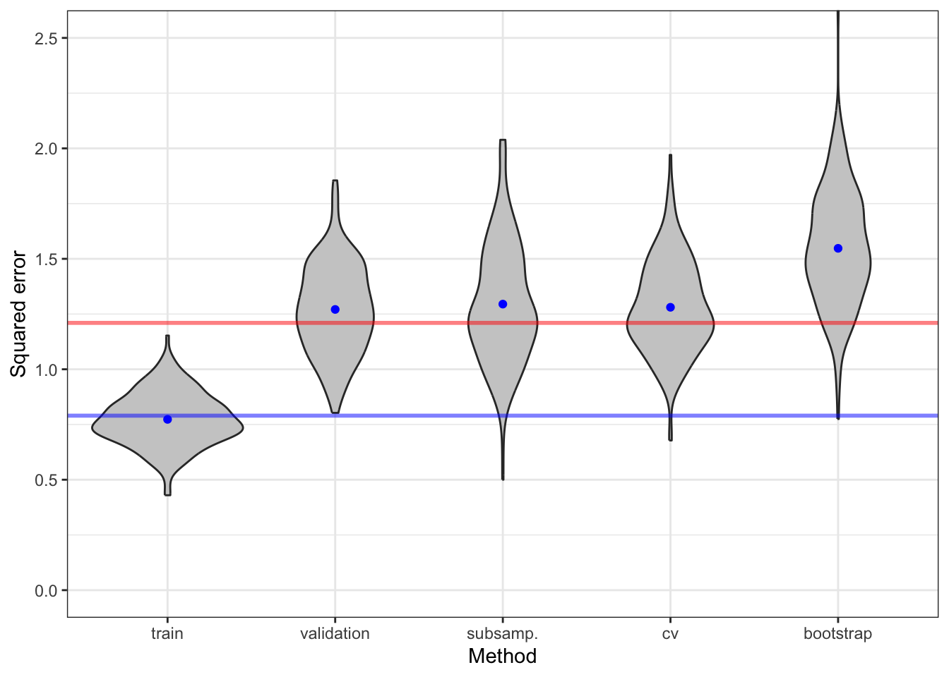

Figure 9.9: Distributions of training error and risk estimators using validation data, subsampling, cross-validation and bootstrapping. All three data splitting methods used \(B = 10\) rounds. The blue line is the expected training error and the red line is the in-sample error.

Method	Mean	SE
train	0.77	0.12
validation	1.27	0.20
subsamp.	1.29	0.27
cv	1.28	0.21
bootstrap	1.55	0.26

Table 9.4: Estimates of mean and standard error for the five different error estimators with \(B = 10\) rounds.

Figure 9.9 shows the distribution of the different error estimators together with the training error. We observe that the training error generally underestimates the expected generalization error as well as the in-sample error. Note that the \(C_p\)-statistic corresponds exactly to the training error plus \(2 p / n = 42 / 100 = 0.42\) in this case.

The different estimates of risk show a considerable variation. A fraction of this variation is due to a random data splitting. By increasing \(B\) we can decrease the variance. Figure 9.10 shows the result of increasing the number of rounds by a factor \(5\) to \(B = 50\).

err_hat <- vector("list", 200)
for(m in seq_along(err_hat)) {
  yx <- sim_yx(n, p0)
  yx_new <- sim_yx(n, p0)
  err_hat[[m]] <- tibble(
    train = train_err(form, yx), 
    validation = val_err(form, yx, yx_new),
    subsamp. = subsamp(form, yx, B = 50),
    cv = cv(form, yx, K = 10, M = 5),
    bootstrap = boot(form, yx, B = 50)
  )
}

Figure 9.10: Distributions of training error and risk estimators using validation data, subsampling, cross-validation and bootstrapping. All three data splitting methods used \(B = 50\) rounds. The blue line is the expected training error and the red line is the in-sample error.

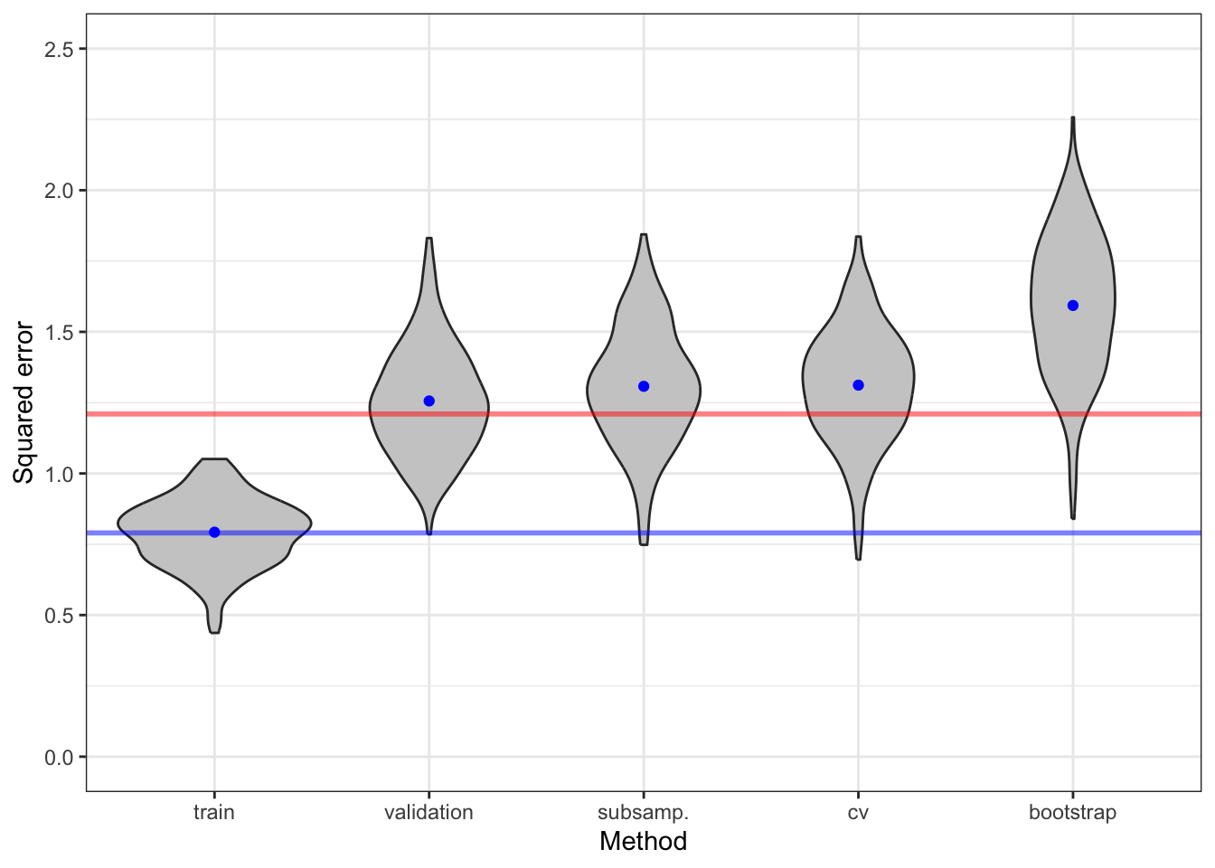
Table 9.4 and Table 9.5 show the means and standard errors for the error estimators. The conclusion is that the increase of \(B\) does decrease the spread of the error estimators’ distributions. This is most pronounced for subsampling and bootstrapping methods. For cross-validation the decrease is detectable, but smaller. We also observe that bootstrapping, as expected, results in a larger error estimate.

Method	Mean	SE
train	0.79	0.12
validation	1.26	0.19
subsamp.	1.31	0.21
cv	1.31	0.20
bootstrap	1.59	0.25

Table 9.5: Estimates of mean and standard error for the five different error estimators with \(B = 50\) rounds.

9.6 Binary model assessment

The framework of risk, generalization error, in-sample error etc. was introduced for a general loss function in the previous sections. The deviance loss – or negative log-likelihood loss – was treated in detail. With a binary response variable there are alternative and widely used methods for assessing the predictive strength of a regression model. This section treats some of the most important ones.

9.6.1 Concordance parameters

A probability model of a binary variable is completely characterized by the probability \(p = P(Y=1)\). For a regression model, this probability will be a function of the predictor, \[ p(x) = P(Y = 1 \mid X= x) = E(Y \mid X = x). \] This is simply the regression function for a binary response.

To give a prediction in the sample space \(\{0,1\}\) we can, for instance, choose a threshold like \(0.5\) and predict that \(Y = 1\) if \(p(X) > 0.5\). It is, however, more informative to know \(p(x)\) than just to know if \(p(x) > 0.5\). The focus is therefore typically on modeling \(p(x)\) rather than just if \(p(x) > 0.5\). It is, moreover, of considerable interest to study predictions generated by a probability model for a range of different values of the threshold instead of just choosing a fixed threshold such as \(0.5\).

For a generalized linear model, \(p(x) = \mu(x^T\beta)\) where \(\mu\) is the mean value function and \(x^T \beta\) is the linear predictor. In this section we will study general prediction models being real valued functions, \(x \mapsto \eta(x) \in \mathbb{R}\), of the predictor. In combination with a choice of mean value function \(\mu : \mathbb{R} \to [0,1]\) a prediction model gives rise to a probability model \[ p(x) = \mu(\eta(x)). \] If the mean value function is strictly monotonely increasing with inverse, \(g\), being the corresponding link function, we observe that \[ p(x) > t \quad \Leftrightarrow \quad \eta(x) > g(t). \]

Definition 9.7 For \(\eta_0\) and \(\eta_1\) independent real valued random variables \[ \mathrm{AUC} = P(\eta_0 < \eta_1) + \frac{1}{2} P(\eta_0 = \eta_1). \]

If the distribution of \(\eta_0\) or \(\eta_1\) is continuous, \[ \begin{align*} \mathrm{AUC} & = P(\eta_0 < \eta_1) \\ & = P(\eta_0 \leq \eta_1). \end{align*} \]

The parameter \(\mathrm{AUC}\) is a concordance parameter, which measures concordance between the distributions of the variables \(\eta_0\) and \(\eta_1\). For \(\mathrm{AUC}\) around \(0.5\) the two distributions are overlapping or in concordance. For \(\mathrm{AUC}\) close to \(1\) or \(0\) the two distributions are well separated.

If \(Y\) is a binary variable and \(\eta(X)\) is a predictor we will be interested in \(\mathrm{AUC}\) for \[ \eta_0 = \eta(X) \mid Y = 0 \quad \text{and} \quad \eta_1 = \eta(X) \mid Y = 1. \] One interpretation of \(\mathrm{AUC}\) is as a quantification of how separated the conditional distributions of \(\eta(X) \mid Y = 0\) and \(\eta(X) \mid Y = 1\) are. A predictor model with \(\mathrm{AUC} \approx 0.5\) will not give accurate predictions of \(Y\) by thresholding \(\eta(X)\). If \(\mathrm{AUC} \approx 1\) it is possible to choose a threshold \(t\) that almost separates the two distributions, so that \(Y\) can be accurately predicted as \(1(\eta(X) > t)\).

Changing the threshold will always change the tradeoff between the type of errors we will make, but the specific choice of threshold does not affect \(\mathrm{AUC}\). This is one of the attractive properties of \(\mathrm{AUC}\). If \(\mathrm{AUC} \approx 0\), the threshold predictor \(1(\eta(X) < t)\) will be an accurate predictor of \(Y\), but we prefer in this case to replace \(\eta(X)\) by \(-\eta(X)\). We will thus always assume that the sign of \(\eta\) is chosen so that larger values of \(\eta(X)\) indicate that \(Y = 1\).

If the distribution functions for \(\eta_0\) and \(\eta_1\) are denoted \(F_0\) and \(F_1\), respectively, then \[ \begin{align*} \mathrm{AUC} & = \int F_0(t) \mathrm{d}F_1(t) - \frac{1}{2} \sum_{t} \Delta F_0(t) \Delta F_1(t) \\ & = \int 1 - F_1(t) \mathrm{d}F_0(t) + \frac{1}{2} \sum_{t} \Delta F_0(t) \Delta F_1(t). \end{align*} \]

Exercises

Exercise 9.1 This exercise is based on the gapminder dataset included in the RwR package. It contains the gross domestic product (GDP) per capita and the average life expectancy at birth (Life) for 139 countries. Figure 9.11 shows a scatter plot of the data.

# RwR version >= 0.3.3
data(gapminder, package = "RwR")
head(gapminder)

# A tibble: 6 × 2
   Life   GDP
  <dbl> <dbl>
1  75.3 12314
2  58.3  7103
3  75.5 14646
4  72.5  7383
5  81.5 41312
6  80.4 43952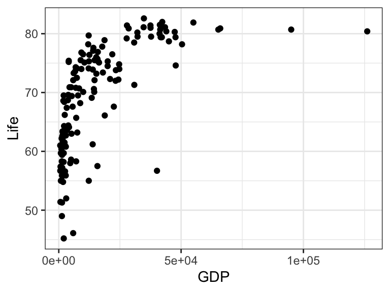

Figure 9.11: Scatter plot of average life expectancy at birth against gross domestic product (GDP).

We will consider a linear model of the form \[ m(x) = E(\mathrm{Life} \mid \mathrm{GDP} = x) = \beta_0 + \sum_{d = 1}^{\mathrm{df}} \beta_d h_d(x) \] where \(m\) is a natural cubic spline. When answering the questions below, use the squared error loss function.

1. Fit the above model with \(1\), \(2\), \(4\), \(8\), and \(16\) degrees of freedom to the gapminder data. Compute the training error for each of the fitted models. Based on a visual inspection of the fitted models, is there any indication of underfitting and overfitting?

2. Compute an estimate of the expected generalisation error using \(10\)-fold cross-validation (with \(M = 1\)). Which model has the best predictive performance?

3. For the model selected above, repeat \(10\)-fold cross-validation \(100\) times and visualize the distribution of the error estimator. How robust are the estimates with respect to the randomness in the data splitting?

4. Redo question 3 above for \(K\)-fold cross-validation with \(K = 5, 10, 20, 50, 100.\) How does the robustness of the estimates change as \(K\) changes? What are the advantages and disadvantages associated with choosing small and large values for K?

Exercise 9.2 Recall from Example 9.1 that a linear estimator is of the form \[ \hat{\boldsymbol{\mu}} = \mathbf{S} \mathbf{Y} \] for an \(\mathbf{X}\)-dependent matrix \(\mathbf{S}\). Here \(\boldsymbol{\mu} = E(\mathbf{Y} \mid \mathbf{X}) \in \mathbb{R}^n\) is the vector of conditional expectations of the response given the predictors.

1. Show that the penalized and weighted least squares estimator, solving the normal equation in Theorem 2.1, is linear and identify the matrix \(\mathbf{S}\).

For the rest of this exercise we assume that the weight matrix is \(\mathbf{W} = I\) and the penalty matrix is diagonal and of the form

\[ \boldsymbol{\Omega} = \lambda \left( \begin{array}{cccc} \omega_1 & 0 & \ldots & 0 \\ 0 & \omega_2 & \ldots & 0 \\ \vdots & \vdots & \ddots & \vdots \\ 0 & 0 & \ldots & \omega_p \end{array} \right) \]

where \(\lambda > 0\). You should think about \(\lambda\) as a tuning parameter that we want to optimize over, while \(\omega_1, \ldots, \omega_p \geq 0\) are fixed penalty weights determining the relative distribution of penalization on the different parameters. We also let \(\hat{\beta}\) and \(\hat{\boldsymbol{\mu}}\) denote the (unpenalized) least squares estimator of \(\beta\) and \(\boldsymbol{\mu}\), respectively.

2. Show that if the model matrix \(\mathbf{X}\) has orthogonal columns¹⁵, then with \[ \gamma_j = \sum_{i=1}^n X_{ij}^2 = \| \mathbf{X}_{\cdot, j} \|^2 \] the squared 2-norm of the \(j\)-th column of \(\mathbf{X}\), the penalized least squares estimator, \(\hat{\beta}_\lambda\), is given by \[ \hat{\beta}_{\lambda,j} = \frac{\gamma_j}{\gamma_j + \lambda \omega_j} \hat{\beta}_j \] and \(\hat{\boldsymbol{\mu}}_\lambda = \mathbf{X} \hat{\beta}_\lambda.\) Show also that the effective degrees of freedom is \[ \mathrm{df}_\lambda = \sum_{j=1}^p \frac{\gamma_j}{\gamma_j + \lambda \omega_j}. \]
3. Show that if \(\omega_1 = \ldots = \omega_p = 1\) then, irrespectively of whether \(\mathbf{X}\) has orthogonal columns, the effective degrees of freedom is \[ \mathrm{df}_\lambda = \sum_{j=1}^p \frac{\gamma_j}{\gamma_j + \lambda}. \] where \(\gamma_1, \ldots, \gamma_p \geq 0\) are the eigenvalues of \(\mathbf{X}^T \mathbf{X}\).

¹⁵ An \(n \times p\) matrix \(\mathbf{X}\) with orthonormal columns satifies that \(\mathbf{X}^T \mathbf{X} = I\), and we may call \(\mathbf{X}\) orthogonal even though it is typically not square \((n > p)\). Here we only assume that the columns are orthogonal implying that \(\mathbf{X}^T \mathbf{X}\) is diagonal.

For the remaining part of this exercise we consider the bike rental data introduced in Section 9.2. Using the poly() function we construct a model matrix with \(p = 7\) orthogonal columns, corresponding to expanding the regression function using orthogonal polynomials of degree \(6\).

data(bike, package = "RwR")
X <- model.matrix(~ poly(Temperature, degrees = 6), data = bike)
beta_hat <- lm.fit(X, bike$Count) |> coefficients()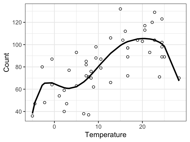

Figure 9.12: Least squares fit of a degree 6 polynomial to the bike rental data.

The least squares estimate is computed above as beta_hat, and the corresponding fitted values are shown in Figure 9.12. For the following questions we take \(\omega_1 = \omega_2 = 0\) and \(\omega_3 = \ldots = \omega_{7} = 1\).

4. Check numerically that X (approximately) has orthogonal columns.
5. Compute an estimate of \(\sigma^2\) based on the least squares estimate \(\hat{\beta}\) of \(\beta\).
6. Implement the computation of \(\hat{\boldsymbol{\mu}}_\lambda\) and \(\mathrm{df}_\lambda\) for a sequence¹⁶ of values of \(\lambda\).
7. Compute \(\mathrm{err}\) for the sequence of \(\lambda\)-values and compute then a sequence of estimates of the in-sample error. Plot the in-sample error against the effective degrees of freedom. What is the best model according to the in-sample error?
8. Implement cross-validation to estimate the expected generalization error. Compare graphically \(\mathrm{err}\), \(\widehat{\mathrm{Err}}_{\mathrm{in}}\) and \(\widehat{\mathrm{Err}}\) as a function of the effective degrees of freedom.

¹⁶ It can be a little tricky to find a suitable sequence. Note that \(\lambda = 0\) gives the least squares estimate and a large value of \(\lambda\) effectively makes \(\hat{\beta}_\lambda = (\hat{\beta}_0, \hat{\beta}_1, 0, \ldots, 0)^T\).

Note: There is a subtle difference between the following two procedures: i) splitting the data and recomputing the model matrix using poly() on a subset of the data; and ii) subsetting the model matrix X that is computed from all data. You may want to explore this difference and think about which of the two procedures is most appropriate.

Exercise 9.3 Let \(\eta_0\) and \(\eta_1\) be independent real valued random variables fulfilling that \[ \eta_1 \overset{\mathcal{D}}{=} \eta_0 + \xi \] for \(\xi \in \mathbb{R}\). That is, the distribution of \(\eta_1\) is a translation by \(\xi\) of the distribution of \(\eta_0\). Assume also that the distribution function, \(F_0\), for \(\eta_0\) is continuous.

1. Show that \[ \mathrm{AUC} = G(\xi) \] where \(G\) is
   \[ G(z) = \int F_0(z + x) \mathrm{d}F_0(x). \]
2. Argue that \(G\) is the distribution function for the distribution of \(\eta_0 - \tilde{\eta}_0\), where \(\tilde{\eta}_0\) is independent of \(\eta_0\) with the same distribution.
3. Show that if \(\eta_0 \sim \mathcal{N}(\mu, \sigma^2)\) then \[ \mathrm{AUC} = \Phi\Big(\frac{\xi}{\sqrt{2}\sigma}\Big). \]

This exercise shows that for Gaussian distributions with the same variance, \(\mathrm{AUC}\) is a monotonely increasing function of the signal-to-noise ratio \(\xi/\sigma\).