13  Interval estimation

Warning

This chapter is still a draft and minor changes are made without notice.

This chapter gives a treatment of the theory and methodology behind interval estimation. While most of the preceeding chapters focus on point estimation of the parameters, the focus of this chapter is on interval estimation of a univariate parameter of interest. The purpose of an interval estimate is to communicate a range of plausible parameter values for the given data rather than a single parameter – and in this way also quantify the uncertainty about a parameter estimate.

13.1 Outline and prerequisites

Standard confidence intervals based on \(Z\)-scores is one way to construct interval estimates, and this method will be treated here in a general context of interval estimation. Likelihood based interval estimation is a different approach to constructing intervals, which will be treated in some detail, and their connection to the standard confidence intervals will be established.

The bootstrap is covered as a general method for standard error estimation and interval calibration to ensure that the computed interval estimators have desired sampling properties.

Some of the theory covered is not specific to regression models, and in the general presentation there are no explicit predictor variables. The observation vector will in the general case be denoted \(\mathbf{Y}\) and consist of \(n\) independent random variables. For regression models this vector then either represents the responses conditionally on the predictors or the joint observation of the responses and predictors.

The chapter primarily relies on the following R packages.

library(RwR)
library(ggplot2)
library(tibble)
library(splines)
library(dplyr)
library(sandwich)
library(lmtest)

13.2 Interval estimators

The focus of the entire chapter is on univariate parameters of interest, and we will denote such a parameter generically by \(\gamma\). It is, in general, a function of the distribution of \(\mathbf{Y}\), which we denote \(\rho\). We can thus abstractly write \(\gamma = \gamma(\rho)\) as a function of \(\rho\). For a particular model, the parameter of interest will often be a very explicit function and it may depend on only aspects of the distribution of \(\mathbf{Y}\).

Example 13.1 (Generalized linear models) The parameter of interest in a generalized linear regression model can be one of the \(\beta\)-parameters, a linear combination of the \(\beta\)-parameters, the linear predictor \(X^T\beta\) or the mean value \(\mu(X^T \beta)\) for a given predictor \(X.\) All these are examples¹ where \(\gamma = \gamma(\beta)\) is actually a function of the regression parameters, in which case a natural estimator of \(\gamma\) is the plug-in estimator \[ \hat{\gamma} = \gamma(\hat{\beta}). \tag{13.1}\]

¹ Examples that only rely on the semiparametric mean-variance specification given by GA1 and GA2. If the parameter of interest is a quantile of \(Y \mid X\), say, it is still a function of \(\beta\), but a plug-in estimator then also relies on GA3.

If \(\hat{\gamma}\) denotes an estimate of \(\gamma\), a simple interval estimate based on \(\hat{\gamma}\) is of the form \(\hat{\gamma} \pm z\), or more generally \[ (\hat{\gamma} - z, \hat{\gamma} - w) \tag{13.2}\] for some choices of \(z \geq w\) (\(w\) is typically negative). It is, however, not obvious how we should choose \(z\) and \(w\), or what properties such an interval has.

We may note that (13.2) can be written as \[ (\hat{\gamma} - z, \hat{\gamma} - w) = \{ \gamma \in \mathbb{R} \mid \hat{\gamma} - \gamma \in (w, z) \}, \] which shows that \[ P( (\hat{\gamma} - z, \hat{\gamma} - w) \ni \gamma ) = P(\hat{\gamma} - \gamma \in (w, z)). \] The probablity² \(P( (\hat{\gamma} - z, \hat{\gamma} - w) \ni \gamma )\) is a coverage probablity of the random interval containing the parameter \(\gamma\). As shown above, this probability can be expressed in terms of the distribution of \(\hat{\gamma} - \gamma\).

² This coverage probability is evaluated for a distribution \(\rho\) of \(\mathbf{Y}\) with \(\gamma(\rho) = \gamma\), and it depends in general on \(\rho\), but see Definition 13.3.

We generalize the simple construction above by introducing the concept of a combinant statistic \(R(\mathbf{Y}, \gamma) \in \mathbb{R}\), which is a function of the observations and the (unknown) parameter of interest. We could, for instance, take \[ R(\mathbf{Y}, \gamma) = \hat{\gamma} - \gamma \] as above.

For a fixed \(\gamma = \gamma_0\), the random variable \(R(\mathbf{Y}, \gamma_0)\) is a statistic, and it is typically a test statistic of the simple hypothesis \(H_0: \gamma = \gamma_0\). We will subsequently refer to \(R\) interchangably as a combinant statistic or just as a statistic, where we use the former when we want to emphasize that \(R\) combines the data and the parameter of interest.

Definition 13.1 For a combinant statistic \(R\) and \(z \geq w\) we define the two-sided interval³ estimate \[ I(\mathbf{Y}) = \{\gamma \in \mathbb{R} \mid R(\mathbf{Y}, \gamma) \in (w, z)\}, \tag{13.3}\] and for \(c \geq 0\) the one-sided interval estimate \[ I(\mathbf{Y}) = \{\gamma \in \mathbb{R} \mid R(\mathbf{Y}, \gamma) < c\}. \tag{13.4}\]

³ We use the term “interval” in a liberal sense. The construction will not result in an interval for all combinant statistics, but we want to avoid introducing an abstract term (such as a “set” or “region” estimate) when most practical constructions will result in intervals.

The definitions above are explicit about the intervals \(I(\mathbf{Y})\) being functions of data only, and we think about the mapping \(\mathbf{Y} \mapsto I(\mathbf{Y})\) as an interval estimator. Specific choices of \(R\), \(w\) and \(z\) (or \(c\)) determine the sampling properties of such estimators. We often aim for constructing intervals with a particular coverage probability.

Definition 13.2 (Coverage and confidence) An interval estimator \(I(\mathbf{Y})\) of the parameter of interest \(\gamma\) has coverage \(1-\alpha\) if \[ P(I(\mathbf{Y}) \ni \gamma) \geq 1 - \alpha. \tag{13.5}\] Such an interval is called a confidence interval with confidence level \(1 - \alpha\).

The definition is, in a certain sense, straightforward, but to fully comprehend it we need to unfold the implicit requirements about the distribution, \(\rho\), of \(\mathbf{Y}\). It is implicit that \(\rho\) belongs to some model, that is, a family of probability distributions, and it is also implicit that \(\gamma(\rho) = \gamma\). The coverage statement about an interval estimator is always relative to a model, and it is possible that an interval estimator has coverage \(1 - \alpha\) relative to one model but not relative to a (larger) model.

When the interval estimator is constructed from the combinant statistic \(R\), the coverage probability can (in the two-sided case) be expressed as \[ P(I(\mathbf{Y}) \ni \gamma) = P(R(\mathbf{Y} , \gamma) \in (w, z)) = R(\rho, \gamma(\rho))((w, z)) \] where \(R(\rho, \gamma(\rho))\) denotes the push-forward measure by \(R\) of the distribution \(\rho\) of \(\mathbf{Y}\).

Definition 13.3 (Pivot) For a given model of the sampling distribution, \(\rho\), of \(\mathbf{Y}\), and for a parameter of interest \(\gamma = \gamma(\rho)\), the combinant statistic \(R\) is said to be a pivot if the distribution of \(R(\mathbf{Y}, \gamma)\) does not depend on \(\rho\). That is, if the probability measure \(R(\rho, \gamma(\rho))\) is independent of \(\rho\).

If we can find a pivot \(R\) then it is particularly easy to construct intervals with guaranteed coverage. If \(w = w_{\alpha}\) and \(z = z_{\alpha}\) are the \(\alpha/2\)- and \((1-\alpha/2)\)-quantiles of the probability distribution \(R(\rho, \gamma(\rho))\), the two-sided interval (13.3) has coverage⁴ \[ P(I(\mathbf{Y}) \ni \gamma) = R(\rho, \gamma(\rho))((w_{\alpha}, z_{\alpha})) = 1 - \alpha / 2 - \alpha/2 = 1 - \alpha \]

⁴ To get exact equality here we assume that the distribution of \(R(\mathbf{Y}, \gamma)\) is continuous. It is always possible to guarantee coverage but perhaps not with exact equality.

For the one-sided interval (13.4) we choose \(c = c_{\alpha}\) to be the \((1-\alpha)\)-quantile of the pivot’s distribution, which likewise gives the coverage guarantee \[ P(I(\mathbf{Y}) \ni \gamma) = R(\rho, \gamma(\rho))((- \infty, c_{\alpha})) = 1 - \alpha. \]

It is, unfortunately, only for a few special models that we can find exact pivots, and in most applications we rely on approximate pivots. Section 13.3.3 deals with several methods for choosing \(w\) and \(z\) or \(c\) to calibrate the interval estimates to have (approximately) a desired coverage probability for a given combinant statistic \(R\). In the following sections we focus on constructions and interpretations of the various statistics that are used in practice for interval estimation.

13.2.1 Standard confidence intervals

With \(\hat{\mathrm{se}}\) any estimate of the standard error⁵ of \(\hat{\gamma}\) we can construct the \(Z\)-statistic \[ Z = \frac{\hat{\gamma}- \gamma}{\hat{\mathrm{se}}}. \] With \(z \geq 0\) and \(w = - z\) in the two-sided interval based on the \(Z\)-statistic we find the corresponding symmetric interval estimate \[ \hat{\gamma} \pm z \cdot \hat{\mathrm{se}} = (\hat{\gamma} - z \cdot \hat{\mathrm{se}}, \hat{\gamma} + z \cdot \hat{\mathrm{se}}). \] We could also use the statistic \(Z^2\) to construct the one-sided interval. If we choose \(c = z^2\) we arrive at the same symmetric interval as above.

⁵ Either as an analytic formula as in Example 13.2 or computed via bootstrapping as in Example 13.6.

Example 13.2 Consider the linear model under the strong modeling assumptions A3 and A5. That is, the joint distribution of the responses given the predictors is a normal distribution. If the parameter of interest is \(\gamma = a^T \beta\), the corresponding \(Z\)-statistic is \[ Z_a = \frac{\hat{\gamma} - \gamma}{\hat{\sigma} \sqrt{a^T(\mathbf{X}^T\mathbf{X})^{-1}a}}. \] Theorem 2.3 implies that its distribution is a \(t_{n-p}\)-distribution, which does not depend on the distribution of \(\mathbf{Y}\) – as long as A3 and A5 are fulfilled. Thus for the model specified by A3 and A5, \(Z_a\) is a pivot and we know its exact distribution. Its square, \[ Z^2_a = \frac{(\hat{\gamma} - \gamma)^2}{\hat{\sigma}^2 a^T(\mathbf{X}^T\mathbf{X})^{-1}a} \] is likewise a pivot, now with an \(F_{1, n-p}\)-distribution.

Quantiles of the \(t_{n-p}\)-distribution (or the \(F_{1, n-p}\)-distribution) depend on the residual degrees of freedom \(\mathrm{df} = n-p\) but are straigthforward to compute. As \(\mathrm{df} \to \infty\), the \(t_{n-p}\)-distribution will converge to a standard normal distribution \(\mathcal{N}(0, 1)\), and the \(F_{1, n-p}\)-distribution will converge to a \(\chi^2_1\)-distribution.

Beyond the normal model specified by the assumptions A3 and A5 we can rarely find the exact distribution of \(Z\)-statistics. However, we typically use the approximation \(Z \overset{\mathrm{approx}}{\sim} \mathcal{N}(0, 1)\), and we then choose \(z = z_{\alpha}\) as the \(1 - \alpha/2\) quantile in the \(\mathcal{N}(0, 1)\)-distribution for the construction of the corresponding intervals. This leads to the standard choice of \(z = 1.96\) to give approximately⁶ 95% coverage.

⁶ We often specifies a nominal coverage of \(1 - \alpha\), which is the coverage probability we aim for, e.g., by computing quantiles in an approximate distribution. The actual coverage probability may then be larger or smaller depending on how good the approximation is.

Formal justification of the approximation \(Z \overset{\mathrm{approx}}{\sim} \mathcal{N}(0, 1)\) is beyond the scope of this chapter. The standard asymptotic arguments are in terms of convergence in distribution when \(n \to \infty\). We emphasize the following important points on the use of the standard intervals based on an estimate of the standard error and the approximation of the distribution of \(Z\) by a normal distribution.

• The approximation of the distribution of the \(Z\)-statistic by a standard normal distribution makes no strong assumptions about the response distribution. It is, in particular, not necessary for the responses to follow a normal distribution.
• The approximation may be poor if the sample size is small, but it is virtually impossible to give useful theoretical guarantees on how large \(n\) should be for the approximation to be adequate. This is instead investigated through simulation studies, but see also the bootstrap methods in Section 13.3.
• Validity of the standard error estimator, \(\hat{\mathrm{se}}\), is crucial for the resulting intervals to have good coverage properties. Poor coverage of a standard interval is often due to model misspecifications that lead to invalid estimators of the standard error, see Section 13.2.3.

13.2.2 Likelihood intervals

The standard confidence intervals quantify rather explicitly the sampling uncertainty of the parameter estimate, and they are constructed with a certain nominal coverage probability in mind. In that way they appear relatively intuitive. They do, however, not really answer the question about which parameters are the most plausible for the given data.

This section introduces likelihood intervals for a parametrized model as a principled way of constructing interval estimates of the most plausible parameter values. While a confidence interval by definition only has a coverage interpretation, likelihood intervals have intrinsic value that can be justified without reference to sampling properties. They are typically calibrated to have desired coverage properties as well but coverage is not their only virtue. The section concludes by showing that standard confidence intervals based on maximum-likelihood estimation are closely related to likelihood intervals.

For a given dataset, the likelihood ratio quantifies the relative evidence in the data of one probability distribution in our statistical model over another. In terms of the generic log-likelihood function \(\ell\) and generic parameter \(\beta\), the difference \[ \ell(\beta_1) - \ell(\beta_2) \] thus quantifies the evidence in the data for \(\beta_1\) over \(\beta_2\). If the difference is positive, there is more evidence for \(\beta_1\), and if it is negative, there is more evidence for \(\beta_2\). The maximum likelihood estimator (MLE) is the parameter – and corresponding probability distribution in our model – for which there is the largest evidence in the data.

We introduce the supremum of the log-likelihood over the parameter space as \[ \ell_{\mathrm{max}} \coloneqq \sup_{\beta} \ell(\beta). \] If the MLE exists and is denoted \(\hat{\beta}^{\mathrm{MLE}}\), we have \(\ell_{\mathrm{max}} = \ell(\hat{\beta}^{\mathrm{MLE}})\), but \(\ell_{\mathrm{max}}\) is well defined even if the MLE is not. To capture abstractly which parameters achieve a likelihood value close to \(\ell_{\mathrm{max}}\) we introduce the likelihood regions as sublevel sets of the negative log-likelihood.

Definition 13.4 (Likelihood regions) If \(\ell_{\mathrm{max}} < \infty\) we define⁷ the family \(\mathcal{L}(c)\) for \(c \geq 0\) of likelihood regions for \(\beta\) as \[ \mathcal{L}(c) = \{\beta \mid 2 (\ell_{\mathrm{max}} - \ell(\beta)) < c \}. \]

⁷ The “2” in the definition is an arbitrary but convenient convention.

The likelihood regions have the following properties⁸:

⁸ And the interpretation that \(\mathcal{L}(c)\) gradually as \(c\) increases includes models for which there is less and less evidence in the data.

• If the MLE exists then \(\hat{\beta}^{\mathrm{MLE}} \in \mathcal{L}(c)\) for all \(c > 0\).
• If \(\beta_1 \in \mathcal{L}(c)\) and \(\beta_2 \not \in \mathcal{L}(c)\) then \(\ell(\beta_1) > \ell(\beta_2)\).
• The likelihood regions increase as a function of \(c\): If \(c_1 < c_2\) then \(\mathcal{L}(c_1) \subseteq \mathcal{L}(c_2)\).

The general (multivariate) likelihood regions are not much easier to comprehend than the likelihood itself, but we can modify the definition to give practically useful interval estimators for a univariate parameter of interest.

Definition 13.5 The profile log-likelihood for a univariate parameter \(\gamma = \gamma(\beta)\) is defined as \[ \ell(\gamma) = \sup_{\beta : \gamma(\beta) = \gamma} \ell(\beta). \] The family of likelihood intervals⁹ for \(\gamma\) is defined as \[ \mathcal{I}(c) = \{\gamma \mid 2 (\ell_{\mathrm{max}} - \ell(\gamma)) < c \}. \]

⁹ As in other cases, the set \(\mathcal{I}(c)\) needs not be an interval, but the terminology becomes less heavy if we accept this slight abuse of the word “interval”.

We note that the likelihood intervals are simply the one-sided interval estimates determined by the combinant statistic \[ R(\mathbf{Y}, \gamma) = 2 (\ell_{\mathrm{max}} - \ell(\gamma)), \] where \(\ell(\gamma)\) is the profile log-likelihood.

The family of likelihood intervals is, just as the family of abstract likelihood regions, a nested family of sets, but as subsets of \(\mathbb{R}\) they are somewhat more comprehensible and easier to communicate. And for any choice of \(c > 0\), parameters in \(\mathcal{I}(c)\) are more plausible than parameters outside of \(\mathcal{I}(c)\).

The obvious question is how the cutoff \(c\) should be chosen if we want to report a single likelihood interval? If we want the interval to be a confidence interval, we need to calibrate \(c\) to yield the desired nominal coverage, and we discuss this in greater detail in Section 13.3.3. A standard choice is \(c = 3.841\) aiming for the interval \(\mathcal{I}(3.841)\) to be a nominal 95% confidence interval by supposing that \(2 (\ell_{\mathrm{max}} - \ell(\gamma))\) approximately follows a \(\chi^2_1\)-distribution¹⁰.

¹⁰ The 95% quantile in the \(\chi^2\)-distribution with one degrees of freedom is \(3.841\).

Absolute interpretations of log-likelihood ratios

There is an alternative to coverage for justifying a choice of the cufoff \(c\) in the construction of likelihood intervals. It is based on an absolute interpretation of log-likelihood ratios. The argument works by constructing a simple analogy to the abstract log-likelihood ratio scale.

The analogy supposes that we draw balls from one of two (infinite) urns, but we don’t known which one it is. One urn has only white balls and the other has half black and half white balls. If we at any time draw a black ball we know for sure that we are drawing from the second urn. But if we have drawn \(b\) white balls without drawing a black we may ask: how strong is the evidence for the “all white” urn over the alternative? The log-likelihood ratio of the “all white” urn over the alternative is \(b \cdot \log(2) \approx 0.69 \cdot b\), and we can regard this number as a quantification of the evidence.

Because the example is simple, we can use it to develop an understanding of the log-likelihood ratio scale. Most would agree that an observation of \(b = 10\) white balls is strong evidence in favor of the “all white” urn, while \(b = 3\) is not. That is, a log-likelihood ratio of \(10 \cdot \log(2) = 6.931\) is “strong evidence”, while a log-likelihood ratio of \(3 \cdot \log(2) = 2.079\) is not. A log-likelihood ratio of \(3.841\) corresponds to \(5.5\) white balls, which seems like moderate evidence for the “all white” urn over the alternative.

The purpose of the simple urn example is to develop a reference by analogy for interpretion of log-likelihood ratios – if we are willing to interpret such ratios absolutely. In that case we can translate a general log-likelihood ratio to an interpretable quantity: the number of white balls drawn. For a thorough treatment of the likelihood principle, promoting this perspective, see the book Statistical Evidence by Richard Royall (1997). The urn example is covered in his Section 1.6. We will not push this interpretation too far, but it is an interesting theoretical perspective.

Royall, Richard M. 1997. Statistical Evidence. Vol. 71. Monographs on Statistics and Applied Probability. Chapman & Hall, London.

Example 13.3 (Generalized linear models) Suppose \(a \in \mathbb{R}^p\) and that the parameter of interest is \(\gamma = a^T \beta\). Suppose first that the MLE, \(\hat{\beta}\), exists and that \(\hat{\gamma} = a^T \hat{\beta}\). The profile log-likelihood over \(\beta\) (ignoring for now the dispersion parameter) is given by \[ \ell(\gamma) = \sup_{\beta: a^T \beta = \gamma} \ell(\beta) = \ell(\hat{\beta}(\gamma)) \] where \(\hat{\beta}(\gamma)\) is the MLE under the linear constraint \(a^T \hat{\beta}(\gamma) = \gamma\). Since we can reparametrize¹¹ the model by \((\tilde{\beta}, \gamma)^T = A \beta\) for an invertible matrix \(A\), the practical computation of \(\hat{\beta}(\gamma)\) is equivalent to computing the MLE in a glm with a fixed offset parameter.

¹¹ With model matrix \(\mathbf{X}\) in the \(\beta\)-parametrization we get that \(\mathbf{X} \beta = \mathbf{X} A^{-1} A \beta = \mathbf{X} A^{-1} (\tilde{\beta}, \gamma)^T\), and the reparametrization corresponds to transforming the model matrix to \(\tilde{\mathbf{X}} = \mathbf{X} A^{-1}\).

The likelihood combinant statistic is recognized as the deviance test statistic \[ 2 (\ell_{\mathrm{max}} - \ell(\gamma)) = D_0(\gamma) - D, \] where \(D_0(\gamma)\) is the deviance corresponding to the affine hypothesis \(H_0: a^T \beta = \gamma\). The computation of the likelihood interval for a fixed \(c\) proceed as follows:

• Compute \(D_0(\gamma)\) for a small number of \(\gamma\)-values around \(\hat{\gamma}\).
• Solve¹² the equation \[ D_0(\gamma) = \hat{\psi} c + D \] using a smooth interpolant of the computed values, e.g., splines.
• Report the two solutions as the interval \[ \mathcal{I}(c) = (\gamma_{\mathrm{lower}}(c), \gamma_{\mathrm{upper}}(c)). \]

¹² We define \(\gamma_{\mathrm{lower}}(c)\) as the largest solution smaller than \(\hat{\gamma}\) and \(\gamma_{\mathrm{upper}}(c)\) as the smallest solution larger than \(\hat{\gamma}\). If there is no solution smaller than \(\hat{\gamma}\) we set \(\gamma_{\mathrm{lower}}(c) = - \infty\), and if there is no solution larger than \(\hat{\gamma}\) we set \(\gamma_{\mathrm{upper}}(c) = \infty\).

The procedure outlined above is implemented via the confint() method for glm objects, see the help pages ?confint.glm and ?profile.glm. The application of profiling for computing likelihood intervals will be demonstrated in Section 13.4.1. The standard confidence intervals given by (6.7) are based on the \(Z\)-statistic \[ Z_a = \frac{\hat{\gamma} - \gamma}{\sqrt{\hat{\psi} a^T (\mathbf{X}^T \hat{\mathbf{W}} \mathbf{X})^{-1}a}} \] as introduced in Section 6.3.2 and corresponding to \[ \hat{\mathrm{se}} = \sqrt{\hat{\psi} a^T (\mathbf{X}^T \hat{\mathbf{W}} \mathbf{X})^{-1}a}. \] They can be computed using confint.lm(). The standard intervals are faster to compute and often similar to the likelihood intervals, but the likelihood intervals often have better coverage properties, in particular for small samples, where they, for good reason, can be rather asymmetric. The likelihood intervals are actually also well defined, computable and potentially informative even if the MLE does not exist, in which case the left or the right (or both) endpoints equal \(-\infty\) or \(+ \infty\), respectively.

Using the distributional approximation¹³, cf. also Equation 6.8, \[ \frac{D_0(\gamma) - D}{\hat{\psi}} \overset{\mathrm{approx}}{\sim} \chi^2_1 \] we may choose \(c\) according to the quantiles of a \(\chi^2_1\)-distribution to achieve the desired nominal coverage. For example, with \(c = 3.841\) the nominal coverage of the likelihood interval is 95%.

¹³ The theoretical justification is known as Wilks’ theorem stating that under suitable regularity assumptions then \[D_0(\gamma) - D \overset{\mathcal{D}}{\to} \psi \chi^2_1\] for \(n \to \infty\) if the model is correctly specified and \(\gamma = a^T \beta\).

If the parameter of interest is \(\mu = \mu(\gamma)\), where \(\mu\) is the mean value function, then the likelihood interval for \(\mu\) (supposing that \(\mu\) is increasing) equals \[ (\mu(\gamma_{\mathrm{lower}}(c)), \mu(\gamma_{\mathrm{upper}}(c))). \] That is, transforming a likelihood interval gives the likelihood interval for the transformed parameter. Contrary to standard confidence intervals it therefore does not matter which scale we choose for constructing likelihood intervals.

If we transform the standard confidence interval \(\hat{\gamma} \pm z \cdot \hat{\mathrm{se}}\) we get the interval \[ (\mu(\hat{\gamma} - z \cdot \hat{\mathrm{se}}), \mu(\hat{\gamma} + z \cdot \hat{\mathrm{se}})). \] This interval will have the same coverage properties on the transformed scale as the standard interval has on the original scale, but it is not a standard interval on the transformed scale.

While it is unproblematic to compute likelihood intervals in practice in the framework of generalized linear models, as outlined above, it is of interest to understand the connection between likelihood intervals and standard confidence intervals for maximum-likelihood estimators. To this end we show the following lemma on profiling a quadratic function.

Lemma 13.1 Let \(\beta = (\alpha^T, \gamma)^T\) with \(\alpha \in \mathbb{R}^{p-1}\) and \(\gamma \in \mathbb{R}\). Let \(h(\beta) = (\hat{\beta} - \beta)^T \mathcal{J} (\hat{\beta} - \beta)\) for a positive definite matrix \(\mathcal{J}\). Then \[ h(\gamma) = \inf_{\alpha} h((\alpha, \gamma)) = \frac{(\hat{\gamma}- \gamma)^2}{(\mathcal{J}^{-1})_{pp}}. \]

Proof. Write the matrix \(\mathcal{J}\) as a block matrix \[ \mathcal{J} = \left(\begin{array}{cc} \mathcal{J}_{11} & \mathcal{J}_{1p} \\ \mathcal{J}_{1p}^T & \mathcal{J}_{pp} \end{array} \right). \] Expanding \(h(\beta)\) in terms of these blocks gives \[ h(\beta) = (\hat{\alpha} - \alpha)^T \mathcal{J}_{11} (\hat{\alpha} - \alpha) + (\hat{\gamma} - \gamma)^2 \mathcal{J}_{pp} + 2(\hat{\alpha} - \alpha)^T \mathcal{J}_{1p} (\hat{\gamma} - \gamma). \]

Minimization over \(\alpha\) for fixed \(\gamma\) gives \[ \hat{\alpha}(\gamma) = \hat{\alpha} + (\hat{\gamma} - \gamma) \mathcal{J}_{11}^{-1} \mathcal{J}_{1p}. \] Plugging this into \(h(\beta)\) gives the profile log-likelihood \[ h(\gamma) = (\hat{\gamma} - \gamma)^2 (\mathcal{J}_{pp} - \mathcal{J}_{1p}^T \mathcal{J}_{11}^{-1} \mathcal{J}_{1p}) . \] By the general formula for inversion of block matrices the lower right corner of \(\mathcal{J}^{-1}\) is \[ (\mathcal{J}^{-1})_{pp} = (\mathcal{J}_{pp} - \mathcal{J}_{1p}^T \mathcal{J}_{11}^{-1} \mathcal{J}_{1p})^{-1}, \] and the result follows.

We can use Lemma 13.1 to connect the log-likelihood intervals to the standard intervals based on the MLE and the observed Fisher information.

For a twice continuously differentiable parametric log-likelihood \(\ell\) and with \(\hat{\beta}^{\mathrm{MLE}}\) in the interior of the (Euclidean) parameter space, a second order Taylor expansion of \(\ell\) around \(\hat{\beta}^{\mathrm{MLE}}\) gives \[ \ell(\beta) \approx \ell_{\max} - \frac{1}{2} (\hat{\beta}^{\mathrm{MLE}} - \beta)^T \mathcal{J}^{\mathrm{obs}} (\hat{\beta}^{\mathrm{MLE}} - \beta). \tag{13.6}\] Here \(\mathcal{J}^{\mathrm{obs}} = - D^2 \ell(\hat{\beta}^{\mathrm{MLE}})\) is the positive (semi)definite observed Fisher information. From (13.6) we get that \[ 2(\ell_{\max} - \ell(\beta)) \approx (\hat{\beta}^{\mathrm{MLE}} - \beta)^T \mathcal{J}^{\mathrm{obs}} (\hat{\beta}^{\mathrm{MLE}} - \beta). \]

OBS: For generalized linear models the dispersion parameter can be ignored for the computation of the MLE of the regression parameters, but it has to be included for the computation of likelihood intervals, cf. also Example 13.3. Similarly, the log-likelihod approximations presented here suppose that the dispersion parameter estimate is included, cf. Theorem 6.1

Suppose that the \(j\)-th coordinate \(\beta_j\) is our parameter of interest and that \(\mathcal{J}^{\mathrm{obs}}\) is positive definite, then Lemma 13.1 gives the following quadratic approximation of the likelihood combinant statistic \[ 2(\ell_{\max} - \ell(\beta_j)) = \inf_{\beta_{-j}} 2(\ell_{\max} - \ell(\beta)) \approx \frac{(\hat{\beta}_j^{\mathrm{MLE}} - \beta_j)^2}{((\mathcal{J}^{\mathrm{obs}})^{-1})_{jj}}, \tag{13.7}\] where the infimum over \(\beta_{-j}\) means over all coordinates in \(\beta\) except \(\beta_j\). We see that the right hand side above equals \(Z^2\) for the \(Z\)-statistic \[ Z = \frac{\hat{\beta}_j^{\mathrm{MLE}} - \beta_j}{\sqrt{((\mathcal{J}^{\mathrm{obs}})^{-1})_{jj}}} \] that corresponds to the standard error estimate \[ \hat{\mathrm{se}} = \sqrt{((\mathcal{J}^{\mathrm{obs}})^{-1})_{jj}}. \]

We emphasize the following key points about likelihood intervals.

• Likelihood intervals have an intrinsic interpretation: the parameter values located centrally in the interval (those that remain in the interval for small \(c\)) are more plausible than those close to the boundaries.
• Likelihood intervals are invariant under reparametrizations: we get the same intervals irrespectively of how the model is parametrized.
• The approximation (13.7) allows us to interpret standard confidence intervals based on the MLE as approximate likelihood intervals. For this reason they inherit the interpretations of likelihood intervals, but the quality of the approximation depends on the parametrization.
• The confint() method for glm objects compute likelihood intervals by profiling. Standard confidence intervals can be computed by calling confint.lm() directly for the glm object.

13.2.3 Robust standard errors

In Chapter 6 on generalized linear models as well as in Chapter 11 on survival models we derived maximum-likelihood estimators of the regression parameters. As discussed in Chapter 6, there is some robustness of the glm estimators toward misspecification of the response distribution. If just the conditional mean and variance are correctly specified, the estimators as well as the statistical inference based on these estimators are still valid. Similarly, the partial likelihood estimator for the proportional hazards model does not require a correct specification of the full response distribution either – the estimators and the statistical inference remain valid as long as the proportional hazards assumption holds and the hazard weights are correctly specified.

In applications we attempt to justify the assumptions we do make via model diagnostics, and we correct misspecifications if possible. In Chapter 7, for example, the first Poisson model of vegetable sales showed a clear but fixable misspecification of the mean-variance relation. It is, however, difficult to eliminate all model misspecifications, either because they are not detectable by the model diagnostics or because they are not easily fixable, Thus we cannot give any guarantees that the model is correctly specified. To partially remedy this we derive in this section analytic methods for standard error estimation that are somewhat robust toward model misspecifications.

We will in this section focus on the regression setup with observations \((X_1, Y_1), \ldots, (X_n, Y_n)\) assumed i.i.d. That is, we make assumption A6 on the joint distribution of the observations. The regression parameter is \(\beta \in \mathbb{R}^p\), and we consider estimators given as solutions to an estimating equation \[ \mathcal{U}(\beta) = \sum_{i=1}^n u(X_i, Y_i, \beta) = 0, \tag{13.8}\] for some estimating function \(u : \mathbb{R}^p \times \mathbb{R} \times \mathbb{R}^p \to \mathbb{R}^p\). In practice, \(\mathcal{U}\) might be a (transposed) score function, but the methods we derive apply to the partial score equation and any other estimating equation.

For a general estimating function we define the target value of the parameter \(\beta\) to be the solution to the equation \[ E(u(X, Y, \beta)) = \int u(x, y, \beta) \rho(dx, dy) = 0, \tag{13.9}\] where \(\rho\) denotes the joint distribution of \((X, Y)\). That is, for any joint distribution we define the parameter \(\beta\) in terms of \(\rho\) via (13.9).

Example 13.4 The estimating equation for a generalized linear model is given in terms of the estimating function \[ \begin{align*} u(X, Y, \beta) & = \theta'(X^T\beta) (Y - \mu(X^T\beta)) X \\ & = \frac{\mu'(X^T\beta)}{\mathcal{V}(\mu(X^T\beta))} (Y - \mu(X^T\beta)) X, \end{align*} \tag{13.10}\] cf. Lemma 6.1 and Theorem 6.1. If the mean is misspecified, the \(\beta\) parameter is determined as the solution to the equation \[ E \left( \frac{\mu'(X^T\beta)}{\mathcal{V}(\mu(X^T\beta))} (E(Y \mid X) - \mu(X^T\beta)) X \right) = 0. \] If the mean is correctly specified as \(E(Y \mid X) = \mu(X^T\beta)\), then this value of \(\beta\) also solves the equation above.

Let \(\hat{\beta}\) denote a solution to the estimating equation \(\mathcal{U}(\beta) = 0\), then by a Taylor expansion of \(\mathcal{U}\) around \(\hat{\beta}\) we find \[ \mathcal{U}(\beta) \approx \mathcal{U}(\hat{\beta}) + \hat{J} (\beta - \hat{\beta}) = \hat{J} (\beta - \hat{\beta}) \] where \[ \hat{J} \coloneqq D_{\beta} \mathcal{U}(\hat{\beta}) = \sum_{i=1}^n D_{\beta} u(X_i, Y_i, \hat{\beta}). \]

The arguments made here are not rigorous but can be made so by sufficiently many regularity assumptions. The important point is to understand the motivation for the sandwich estimator defined below as a robust variance estimator.

Since \(E(u(Y_i, X_i, \beta)) = 0\) the central limit theorem implies that \[ \frac{1}{n} \hat{J} (\hat{\beta} - \beta) \approx \frac{1}{n} \sum_{i=1}^n u(X_i, Y_i, \beta) \overset{\mathrm{as}}{\sim} \mathcal{N}(0, C_1 / n) \] where \[ C_1 \coloneqq V(u(X, Y, \beta)) = E(u(X, Y, \beta)u(X, Y, \beta)^T). \] With \[ \hat{C} \coloneqq \sum_{i=1}^n u(X_i, Y_i, \hat{\beta}) u(X_i, Y_i, \hat{\beta})^T \] then \(\hat{C} / n\) is an estimator of \(C_1\), and with \(Z \sim \mathcal{N}(0, I)\) we arrive at the distributional approximation \[ \hat{\beta} - \beta \overset{\mathcal{D}}{\approx} n \hat{J}^{-1} (\hat{C} / n^2)^{1/2} Z = \hat{J}^{-1} \hat{C}^{1/2} Z \sim \mathcal{N}(0, \hat{J}^{-1} \hat{C} \hat{J}^{-T}). \] The estimator \[ \hat{\Sigma} \coloneqq \hat{J}^{-1} \hat{C} \hat{J}^{-T} \tag{13.11}\] of the asymptotic covariance matrix is known as the sandwich estimator.

If the estimating equation is a score equation, Bartlett’s second identity states that when the model is correctly specified \(C_1 = E(D_\beta u(X, Y, \beta))\), in which case \(\hat{C} \hat{J}^{-T} \approx I\). So for a correctly specified model we can simply use the inverse of the observed Fisher information \(\hat{J}^{-1}\) as an estimator of the asymptotic covariance matrix. The sandwich estimator is an alternative that does not assume Bartlett’s second identity, and it is (somewhat) robust against model misspecifications.

Example 13.5 For the estimating equation based on generalized linear models, \[ \hat{J} = \mathcal{J}^{\mathrm{obs}} = \mathbf{X}^T \hat{\mathbf{W}}^{\mathrm{obs}} \mathbf{X}, \] where \(\hat{\mathbf{W}}^{\mathrm{obs}}\) is the diagonal matrix given by Equation 6.1 evaluated in \(\hat{\beta}\). We also find that \[ \hat{C} = \sum_{i=1}^n \frac{(\hat{\mu}'_i)^2}{\mathcal{V}(\hat{\mu}_i)^2}(Y_i - \hat{\mu}_i)^2 X_i X_i^T = \mathbf{X}^T \widetilde{\mathbf{W}} \mathbf{X}, \] where \(\widetilde{\mathbf{W}}\) is diagonal with entries \[ \tilde{w}_{ii} = \frac{(\hat{\mu}'_i)^2}{\mathcal{V}(\hat{\mu}_i)^2}(Y_i - \hat{\mu}_i). \]

For generalized linear models we typically use the estimated Fisher information rather than the observed Fisher information, that is, we replace \(\hat{\mathbf{W}}^{\mathrm{obs}}\) by \(\hat{\mathbf{W}}\), which is the diagonal weight matrix with weights \[ \hat{w}_{ii} = \frac{(\hat{\mu}'_i)^2}{\mathcal{V}(\hat{\mu}_i)}. \] We then arrive at the sandwich estimator for the (asymptotic) covariance matrix of the glm estimator: \[ \tilde{\Sigma} = (\mathbf{X}^T \hat{\mathbf{W}} \mathbf{X})^{-1} (\mathbf{X}^T \widetilde{\mathbf{W}} \mathbf{X}) (\mathbf{X}^T \hat{\mathbf{W}} \mathbf{X})^{-1}. \tag{13.12}\]

The weights \(\tilde{w}_{ii}\) can be represented in two ways in terms of \(\hat{w}_{ii}\) and either the Pearson residuals or the working residuals. First we see that \[ \tilde{w}_{ii}= \hat{w}_{ii} \frac{(Y_i - \hat{\mu}_i)^2}{\mathcal{V}(\hat{\mu}_i)}, \tag{13.13}\] where the weights \(\hat{w}_{ii}\) are multiplied by the squared Pearson residual, and then that \[ \tilde{w}_{ii} = \left( \hat{w}_{ii} \frac{Y_i - \hat{\mu}_i}{\hat{\mu}_i'} \right)^2, \tag{13.14}\] where the weights \(\hat{w}_{ii}\) are multiplied by the working residuals and everything is then squared.

Note that if the mean is correctly specified (GA1 holds) then \(E((Y_i - \mu_i)^2 \mid X_i ) = V(Y_i \mid X_i)\), and¹⁴ \[ E(\tilde{w}_{ii} \mid X_i) \approx \hat{w}_{ii} \frac{V(Y_i \mid X_i)}{\mathcal{V}(\hat{\mu}_i)}. \] If the variance function is also correctly specified (GA2 holds), then \(V(Y_i \mid X_i) = \psi \mathcal{V}(\mu_i)\) and \(E(\tilde{w}_{ii} \mid X_i) \approx \psi \hat{w}_{ii}\), and the sandwich formula (13.12) will be relatively close to \(\hat{\psi} (\mathbf{X}^T \hat{\mathbf{W}} \mathbf{X})^{-1}\). But if either or both of GA1 or GA2 are wrong, the weights \(\tilde{w}_{ii}\) can be interpreted as adjustments for the misspecification of the model.

¹⁴ We don’t get exact equality because the weights are computed using the estimated parameters.

Standard error estimates using the sandwich estimator can be computed using the sandwich R package. We can use these standard error estimates for construction of standard confidence intervals. This will be illustrated in Section 13.4.2.

It almost sounds too good to be true that we can compute valid confidence intervals without making any model assumptions – and in a certain sense it is, as argued forcefully by Freedman (2006). If the mean value is wrongly specified, it is often not possible to interpret the target parameter, which makes it very unclear what the value of the confidence interval is – even if it technically has the correct coverage. Thus the robust intervals for generalized linear models are primarily useful when GA2 might be violated but GA1 holds.

Freedman, David A. 2006. “On The So-Called ‘Huber Sandwich Estimator’ and ‘Robust Standard Errors’.” The American Statistician 60 (4): 299–302.

13.3 Bootstrap

Bootstrapping is an alternative to asymptotic theory, or other theoretical arguments, for computing approximations of the sampling distribution of a statistic or a combinant statistic of interest. We will in this section focus on how bootstrapping can be used to construct confidence intervals for a parameter of interest. We will first describe the basic resampling framework of bootstrapping and outline various bootstrap resampling algorithms before we discuss in greater detail how the bootstrap is used for calibration of interval estimators.

13.3.1 Bootstrap basics

Bootstrapping is usually based on simulations rather than analytic methods. Specifically, on resampling of new datasets.

The two basic steps of the bootstap are:

1. Sample \(B\) independent new datasets \(\mathbf{Y}_1^*,\ldots,\mathbf{Y}_B^*\).
2. Compute the statistic of interest from each resampled data set.

The statistic is typically either a parameter estimator, a test statistic or a combinant statistic. Its resampling distribution is also known as its bootstrap distribution.

From the \(B\) datasets it is possible to compute estimates of descriptive quantities of the bootstrap distribution, such as its standard deviation, the bias of an estimator, or quantiles of a combinant statistic. Section 13.3.3 discusses the principles behind using the bootstrap distribution to calibrate combinant-based intervals to have the desired coverage. These principles have nothing to do with the actual resampling but have everything to do with how well the distribution we resample from approximates the target sampling distribution. We postpone this discussion until we have developed the more operational resampling aspect of bootstrapping.

In practice, everything we are interested in about the bootstrap distribution is estimated from the empirical distribution based on the \(B\) resampled datasets. The finite number \(B\) of resampled datasets introduces a sampling error, and \(B\) should be chosen as large as possible to avoid this error to influence on the reported results. An appropriate choice is dictated by the trade-off between computational costs and the accuracy required by the application. We will give more advice on the choice of \(B\) below depending on the specific application of the bootstrap.

One of the most basic usages of the bootstrap is as a tool to compute an estimate of the standard error of an estimator.

Example 13.6 (Bootstrap standard error estimation) Let \(\gamma\) denote the parameter of interest and let \(\hat{\gamma} = \hat{\gamma}(\mathbf{Y})\) denote the estimate based on the the data \(\mathbf{Y}\). From the resampled data \(\mathbf{Y}_1^*,\ldots,\mathbf{Y}_B^*\) we compute reestimates \[ \hat{\gamma}_b^* = \hat{\gamma}(\mathbf{Y}_b^*) \] of the parameter of interest. Then we estimate the standard error of \(\hat{\gamma}\) as \[ \hat{\mathrm{se}} = \sqrt{\frac{1}{B-1} \sum_{b=1}^B (\hat{\gamma}_b^* - \overline{\gamma}^*)^2} \] with \(\overline{\gamma}^* = \frac{1}{B} \sum_{b=1}^B \hat{\gamma}_b^*\). We can use \(\hat{\mathrm{se}}\) to construct the standard 95% confidence interval \[ \hat{\gamma} \pm 1.96 \cdot \hat{\mathrm{se}}. \] For estimation of the standard error, \(B = 200\) is usually enough for acceptable precision.

13.3.2 Bootstrap algorithms

The two major resampling algorithms are known as nonparametric and parametric bootstrapping. They have an abstract form and some specific variants for regression models. A third resampling algorithm, known as residual resampling, is specific to regression models, and the wild bootstrap, that we will not cover, should also be mentioned as a regression specific bootstrap algorithm.

Nonparametric bootstrapping

Nonparametric bootstrapping does not require a parametric model, but it does require some distributional assumptions that allow us to sample new data sets from an empirical distribution. In the abstract formulation the assumption is that \(\mathbf{Y} = (Y_1, \ldots, Y_n)\) with \(Y_1, \ldots, Y_n\) i.i.d. Each resampled data set is obtained by sampling \(n\) observations from \(Y_1, \ldots, Y_n\) with replacement. This is in practice carried out by sampling \(n\) independent indices uniformly from \(\{1, \ldots, n\}\). A resampled data set \[ \mathbf{Y}^* = (Y_{1}^*, \ldots, Y_{n}^*) \] thus consists of \(n\) i.i.d. observations from the empirical distribution \[ \sum_{i=1}^n \delta_{Y_i}. \]

In a regression context the response variables \(Y_1, \ldots, Y_n\) are not identically distributed conditionally on the predictors. Thus we cannot just resample the responses with replacement, say. But under assumption A6 the pairs \((Y_i, X_i)\) are i.i.d.. This may be a resonable assumption when the predictors and the response are observed jointly, while it makes little sense for an experiment where the predictors are fixed by a design.

Pair sampling for nonparametric bootstrapping in a regression setup proceeds under assumption A6 by resampling \(n\) pairs independently from the dataset \((X_1, Y_1), \ldots, (X_n, Y_n)\) with replacement. That is, the resampled dataset consists of \(n\) i.i.d. observations \((X_1^*, Y_1^*), \ldots, (X_n^*, Y_n^*)\) from the empirical distribution \[ \sum_{i=1}^n \delta_{(X_i, Y_i)}. \] The actual implementation is still done in practice by sampling \(n\) independent indices uniformly from \(\{1, \ldots, n\}\).

Parametric bootstrapping

Parametric bootstrapping amounts to resampling data from the parametrically specified model of the data. In the abstract formulation the distribution of \(\mathbf{Y}\) is assumed to be in a parametrized family \(\rho_{\beta}\) of probability measures, and \(\hat{\beta}\) is the estimate of \(\beta\) based on \(\mathbf{Y}\). Then we resample \(\mathbf{Y}^*\) as \(n\) i.i.d. observations from \(\rho_{\hat{\beta}}\).

In the regression setup we can do parametric bootstrapping either conditionally or unconditionally on the predictors. Both require the strong distributional model assumption GA3.

Conditional parametric bootstrapping amounts to resampling the responses \(\mathbf{Y}^* = (Y_1^*, \ldots, Y_n^*)\) under assumption A5. That is, we resample the coordinates \(Y_i^* \mid X_i\) independently from the fitted exponential dispersion model \(\mathcal{E}(\theta(\hat{\eta}_i), \nu_{\hat{\psi}})\). Contrary to nonparametric pair sampling, this form of bootstrapping does not assume A6 and makes good sense for a designed experiment.

Unconditional parametric bootstrapping requires additionally a parametric model of the predictor distribution. Resampling proceeds under assumption A6 and consists of two steps:

1. Sample \(\mathbf{X}^* = (X_1^*, \ldots, X_n^*)\) i.i.d. from the fitted predictor distribution. Set \(\hat{\eta}_i^* = (X_i^*)^T \hat{\beta}\).
2. Sample \(Y_1^*, \ldots, Y_n^*\) given \(\mathbf{X}^*\) independently with \(Y_i^* \mid \mathbf{X}^* \sim \mathcal{E}(\theta(\hat{\eta}_i^*), \nu_{\hat{\psi}})\).

We would rarely want to do unconditional parametric bootstrapping as this requires a full model of the predictors. But we could implement a hybrid algorithm where step 1. above is replaced by resampling the predictors from the empirical distribution. That is, the resampling of the predictors is nonparametric, but the resampling given the predictors is parametric.

Residual resampling

Residual resampling is a version of nonparametric bootstrapping for regression models where residuals and not responses are resampled. Just as conditional parametric bootstrapping above, this algorithm only requires assumption A5 and makes sense for designed experiments in particular.

Residual resampling is simplest to formulate for the additive noise model where \[ Y_i = \mu(X_i^T \beta) + \varepsilon_i \] with \(\varepsilon_1, \ldots, \varepsilon_n\) i.i.d. given \(\mathbf{X}\). In this case the raw residuals are \[ \hat{\varepsilon}_i = Y_i - \mu(X_i^T\hat{\beta}) = Y_i - \hat{\mu}_i. \] We resample a new data set by resampling raw residuals with replacement. That is, a resampled response vector \(\mathbf{Y}^* = (Y_{1}^*, \ldots, Y_{n}^*)\) is constructed as follows:

1. Sample the residuals \(\varepsilon_1^*,\ldots, \varepsilon_n^*\) independently from \(\hat{\varepsilon}_1,\ldots,\hat{\varepsilon}_n\) with replacement.
2. Set \(Y_i^* = \hat{\mu}_i + \varepsilon^*_i\) for \(i = 1, \ldots, n.\)

For residual resampling the predictor variables are held fixed just as for conditional parametric bootstrapping. The resampling of residuals is in practice carried out as for the other nonparametric bootstrapping procedures by sampling indices uniformly. It is possible to combine the residual resampling above with a nonparametric bootstrap resampling of the predictors – if we are willing to make the stronger assumption A6.

It is not straightforward to extend residual resampling to all generalized linear models. We would need an one-to-one map \(t_\mu : \overline{\mathcal{J}} \to \mathbb{R}\) with the property that the distribution of \(\varepsilon = t_\mu(Y)\) and \(X\) are independent when \(E(Y \mid X) = \mu\) and \(V(Y \mid X) = \psi \mathcal{V}(\mu)\). For the additive noise model this map is \(t_\mu(y) = y - \mu\). If we can find such a map \(t_\mu\), the residuals are defined as \(\hat{\varepsilon}_i = t_{\hat{\mu}_i}(Y_i)\) and we replace step 2. above by

2. Set \(Y_i^* = t_{\hat{\mu}_i}^{-1}(\varepsilon^*_i)\) for \(i = 1, \ldots, n.\)

The additive noise model can be generalized to the model where \[ Y_i = \mu(X_i^T \beta) + \sqrt{\mathcal{V}(\mu(X_i^T \beta))} \varepsilon_i \tag{13.15}\] with \(\varepsilon_1, \ldots, \varepsilon_n\) i.i.d. given \(\mathbf{X}\). Then we can take \[ t_{\mu}(y) = \frac{y - \mu}{\sqrt{\mathcal{V}(\mu)}}. \] The resulting resampled residuals are the Pearson residuals, but the corresponding bootstrap distribution is only approximating the sampling distribution of the responses correctly for the specific model (13.15).

13.3.3 Bootstrap calibration

The classical usage of the bootstrap for interval estimation is to compute an approximation to the distribution of a combinant statistic \(R\). This approximation can then be used to calibrate an \(R\)-based interval construction to have the desired (nominal) coverage.

The bootstrap was introduced in a seminal paper by Bradley Efron (1979), who very clearly presented the basic ideas. The goal is to approximate the distribution of a combinant statistic \(R(\mathbf{Y}, \gamma)\) when \(\mathbf{Y} \sim \rho\) for an unknown \(\rho\) with \(\gamma = \gamma(\rho)\) a functional of \(\rho\). The main principle behind bootstrapping is the distributional approximation \[ R(\mathbf{Y}, \gamma) \overset{\mathcal{D}}{\approx} R(\mathbf{Y}^*, \hat{\gamma}) \tag{13.16}\] with \(\mathbf{Y}^* \sim \hat{\rho}\). Here \(\hat{\rho}\) is an estimate of \(\rho\) based on \(\mathbf{Y}\) and \(\hat{\gamma}\) is an estimate of \(\gamma\). That is, we approximate the unknown sampling distribution of \(R(\mathbf{Y}, \gamma)\) by the known bootstrap distribution of \(R(\mathbf{Y}^*, \hat{\gamma})\).

Efron, B. 1979. “Bootstrap Methods: Another Look at the Jackknife.” The Annals of Statistics 7 (1): 1–26.

Note that it is possible for \(\hat{\gamma} \neq \gamma(\hat{\rho})\). Indeed, \(\hat{\gamma}\) is in a regression context typically a plug-in estimate \(\gamma(\hat{\beta})\) based on the parametric estimate of \(\beta\), while \(\hat{\rho}\) is (derived from) an empirical distribution.

Example 13.7 (Bootstrapping a pivot) Suppose that we have a parametrized model \(\rho_{\beta}\) and \(\gamma = \gamma(\beta)\). With \(\hat{\beta}\) the estimate of \(\beta\) we can use the plug-in estimates \(\hat{\gamma} = \gamma(\hat{\beta})\) and \(\hat{\rho} = \rho_{\hat{\beta}}\) of \(\gamma\) and \(\rho\), respectively. The statistic \(R\) is a pivot if the sampling distribution of \[ R(\mathbf{Y}, \gamma(\beta)), \qquad \mathbf{Y} \sim \rho_{\beta} \] does not depend upon \(\beta\). If \(R\) is a pivot, the approximation (13.16) is a distributional identity. That is, there is no approximation error, and the sampling distribution can be computed exactly as the distribution of \(R(\mathbf{Y}^*, \gamma(\hat{\beta}))\) for \(\mathbf{Y}^* \sim \rho_{\hat{\beta}}\).

The standardized \(Z\)-score in Theorem 2.3, see also Example 13.2, is an example of a pivot, whose distribution can be found analytically. The analytic and the parametric bootstrap solutions coincide in this case.

The bootstrap was inspired, in particular, by jackknife methods, which, among other things, had been introduced earlier for nonparametric bias and variance estimation. Like jackknife methods, bootstrapping was developed in a nonparametric framework, and the original resampling algorithm was nonparametric bootstrapping. For nonparametric bootstrapping we cannot expect \(R\) to be a pivot, though, and a systematic study of the “degree of pivotality” of different statistics is beyond the scope of this book. The take-home message is that the distribution of the statistic \(R\) should be as insensitive as possible to the joint approximation error \((\hat{\rho}, \hat{\gamma}) \approx (\rho, \gamma)\) for the bootstrap to be accurate and useful.

We present a couple of examples to illustrate how the bootstrap is used in practice for various combinant statistics for the calibration and computation of interval estimates.

Example 13.8 The simplest combinant statistic is arguably \[ R(\mathbf{Y}, \gamma) = \hat{\gamma} - \gamma. \] With \(w_{\alpha}\) and \(z_{\alpha}\) the \(\alpha/2\) and \(1-\alpha/2\) quantiles for \(R\), the nominal level \((1-\alpha)\)-confidence interval is \[ \{\gamma \in \mathbb{R} \mid \hat{\gamma} - \gamma \in (w_{\alpha},z_{\alpha})\} = (\hat{\gamma} - z_{\alpha},\hat{\gamma} - w_{\alpha}). \]

Estimates, \(\hat{w}_{\alpha}\) and \(\hat{z}_{\alpha}\), of the quantiles are obtained as the empirical quantiles for the bootstrapped sample \[ \hat{\gamma}_1^*- \hat{\gamma},\ldots,\hat{\gamma}_B^*- \hat{\gamma}. \] Here \(\hat{\gamma}_b^* = \hat{\gamma}(\mathbf{Y}_b^*)\) is the estimate based on the \(b\)-th resampled data set \(\mathbf{Y}_b^*\). This is a simple procedure, but approximate pivotality of \(R\) is often questionable.

Example 13.9 With \(\hat{q}_{\alpha}\) and \(\hat{r}_{\alpha}\) denoting the \(\alpha/2\) and \((1-\alpha/2)\)-quantiles for the empirical distribution of the reestimates \[ \hat{\gamma}_1^*,\ldots,\hat{\gamma}_B^*, \] the percentile confidence interval is defined simply as \[ (\hat{q}_{\alpha},\hat{r}_{\alpha}). \] There are theoretical arguments justifying this interval if there exists a monotone transformation of \(\hat{\gamma}\), which is a pivot and whose distribution is symmetric. We may observe that \(\hat{w}_{\alpha} = \hat{q}_{\alpha} - \hat{\gamma}\) and \(\hat{z}_{\alpha} = \hat{r}_{\alpha} - \hat{\gamma}\), and the confidence interval based on the simple combinant statistic equals
\[ (2\hat{\gamma} - \hat{r}_{\alpha},2\hat{\gamma} - \hat{q}_{\alpha}). \] This interval is generally different from the percentile interval, but if the distribution of \(\hat{\gamma}\) is close to being symmetric around¹⁵ \(\gamma\), the two intervals are almost identical. The percentile interval has the nice property of being invariant to monotone parameter transformations, but its actual coverage is sometimes poor.

¹⁵ It often is!

Example 13.10 The combinant statistic can be the (profile) negative log-likelihood \[ R(\mathbf{Y}, \gamma) = 2(\ell_{\mathrm{max}} - \ell(\gamma)). \] From the bootstrap sample \[ 2(\ell_{\mathrm{max}, 1}^* - \ell(\hat{\gamma})), \ldots, 2(\ell_{\mathrm{max}, B}^* - \ell(\hat{\gamma})) \] we compute the estimate \(\hat{c}_{\alpha}\) of the \((1-\alpha)\)-quantile, and the corresponding likelihood interval for \(\gamma\) with nominal coverage \(1-\alpha\) becomes \[ \{ \gamma \mid 2(\ell_{\mathrm{max}} - \ell(\gamma)) < \hat{c}_{\alpha}\}. \]

Example 13.11 If we have an analytic estimate of the standard error, we can also bootstrap the \(Z\)-statistic or \(Z^2\). With
\[ R(\mathbf{Y}, \gamma) = \frac{(\hat{\gamma} - \gamma)^2}{\hat{\mathrm{se}}^2} \] the bootstrap sample becomes \[ \frac{(\hat{\gamma}^*_1 - \hat{\gamma})^2}{(\hat{\mathrm{se}_1^*})^2}, \ldots, \frac{(\hat{\gamma}^*_B - \hat{\gamma})^2}{(\hat{\mathrm{se}_B^*})^2}, \] which we as above use to estimate \(\hat{c}_{\alpha}\) as the empirical \((1-\alpha)\)-quantile. The corresponding confidence interval for \(\gamma\) then becomes
\[ \{ \gamma \mid (\hat{\gamma} - \gamma)^2 < \hat{c}_{\alpha} {\hat{\mathrm{se}}^2}\} = \hat{\gamma} \pm \sqrt{\hat{c}_{\alpha}} \cdot \hat{\mathrm{se}}. \]

In all the examples above, the actual coverage will be close to \(1 - \alpha\) whenever the combinant statistic is sufficiently close to being a pivot and \(B\) is large enough. The bootstrap does not work without assumptions, but it does not rely on strong distributional approximations, such as a \(\mathcal{N}(0, 1)\)- or a \(\chi^2_1\)-distribution of the combinant statistic.

We should note that if we only use the bootstrap to estimate the standard error, the resulting standard interval, as in Example 13.6, still supposes that the \(Z\)-statistic \[ \frac{\hat{\gamma} - \gamma}{\hat{\mathrm{se}}} \] is approximately \(\mathcal{N}(0,1)\)-distributed. It is possible to use the bootstrap for both estimating the standard error and for calibrating the interval based on the \(Z\)-statistic, but it requires nested bootstrapping with heavy computational costs.

As mentioned in Example 13.6, if we only want an estimate of the standard error, \(B = 200\) is usually large enough. If we want to estimate quantiles to calibrate intervals to have 95% coverage, the rule of thumb is to take \(B=999\). If we aim for larger coverage¹⁶ we need to take \(B\) even larger to get an acceptable relative accuracy of the empirical quantiles.

¹⁶ From a testing perspective this is equivalent to computing a more accurate \(p\)-value for testing hypotheses about \(\gamma\).

13.4 Advertising revisited

We revisit the advertising case from Chapter 7. The main focus in this section is to compute a confidence interval for the effect of advertising as expressed by the regression parameter for the categorical variable ad.

We first load the and clean the data as in Chapter 7.

data(vegetables, package = "RwR")
vegetables <- filter(vegetables, !is.na(discount), week != 2)

13.4.1 Model based intervals

We fit a Poisson model with the same formula as used with the gamma model in Section 7.4 (with a natural cubic spline expansion of discount). We then compute a standard confidence interval for the regression parameter associated with the variable ad via confint.lm(). The default nominal coverage of all confidence intervals is 95%.

form <- sale ~ offset(log(normalSale)) + store  + ad + 
  ns(discount, knots = c(20, 30, 40), Boundary.knots = c(0, 50)) - 1
vegetables_glm <- glm(form, family = poisson, data = vegetables)
int_to_tib <- function(x, name) 
 tibble(interval = name, lower = x[1], upper = x[2])
ad_int <- confint.lm(vegetables_glm, "ad1") |> 
    int_to_tib("Pois standard")
ad_int 

# A tibble: 1 × 3
  interval      lower upper
  <chr>         <dbl> <dbl>
1 Pois standard 0.446 0.563

The vegetables_glm object is of class glm. It means that when the generic function confint() is called with this object as argument, it calls the method confint.glm() for this class. This method computes likelihood intervals by profiling. We compare the resulting confidence interval to the standard confidence interval.

confint(vegetables_glm, "ad1") |> 
    int_to_tib("Pois likelihood") |>
    add_row(ad_int) -> ad_int
ad_int

# A tibble: 2 × 3
  interval          lower   upper
  <chr>             <dbl>   <dbl>
1 Pois likelihood 0.44580 0.56305
2 Pois standard   0.44573 0.56319

We find that the two intervals are identical up to the fourth decimal. Thus for this example there is for practical purposes no difference between the two intervals.

The interval produced by either method is fairly narrow and identifies a clearly significant positive association between advertising and sales. However, as discussed in Chapter 7, we know that the Poisson model is misspecified so we have no reason to expect that this construction with nominal level 95% has 95% actual coverage.

Due to the overdispersion and/or the misspecification of the variance function by the Poisson model, we fit alternative models with the same mean value specification (same formula and same link function) but using the quasi Poisson family as well as the gamma model. For each model fit we then compute both standard and likelihood intervals. The results are shown in Table 13.1.

vegetables_glm_quasi <- glm(form, family = quasipoisson, data = vegetables)
vegetables_glm_gamma <- glm(form, family = Gamma("log"), data = vegetables)
confint.lm(vegetables_glm_quasi, "ad1") |> 
    int_to_tib("Q-Pois standard") |>
    add_row(ad_int) -> ad_int
confint(vegetables_glm_quasi, "ad1") |> 
    int_to_tib("Q-Pois likelihood") |>
    add_row(ad_int) -> ad_int
confint.lm(vegetables_glm_gamma, "ad1") |> 
    int_to_tib("Gamma standard") |>
    add_row(ad_int) -> ad_int
confint(vegetables_glm_gamma, "ad1") |> 
    int_to_tib("Gamma likelihood") |>
    add_row(ad_int) -> ad_int

interval	lower	upper
Gamma likelihood	0.10245	0.57064
Gamma standard	0.10891	0.56131
Q-Pois likelihood	0.30361	0.70461
Q-Pois standard	0.30367	0.70525
Pois likelihood	0.44580	0.56305
Pois standard	0.44573	0.56319

Table 13.1: Six different computations of confidence intervals with nominal coverage 95%.

The intervals based on the quasi Poisson family are unsurprisingly somewhat wider because the estimated dispersion parameter is somewhat larger than \(1\). The likelihood interval is again almost identical to the standard interval for the quasi Poisson family, because it is also just a rescaling by the estimated dispersion parameter.

The intervals for the gamma model are even wider and are furthermore skewed toward zero. There is a slightly larger difference between the standard interval and the likelihood interval for the gamma model, but it is still a relatively small difference.

13.4.2 Robust standard errors

We turn to standard confidence intervals based on the sandwich estimator of the asymptotic covariance matrix. We first show how to compute both the ordinary estimate of the asymptotic covariance matrix and the robust estimate by using the formulas explicitly, and then we show below how to use the sandwich package.

We first compute the estimates of the asymptotic covariance matrices by extracting all the relevant components from the glm object. We illustrate these computations using the Poisson model. The weights \(\hat{w}_{ii}\) are extracted using the weights() function with argument¹⁷ type = "working", and we compute the estimated Fisher information matrix in terms of the weights and the model matrix.

¹⁷ These are actually the weights from the last (\(m\)-th) iteration of the IWLS algorithm. That is, they are computed from \(\hat{\beta}_{m-1}\), and they are not numerically identical to weights computed from the returned estimate \(\hat{\beta}_{m}\).

w_hat <- weights(vegetables_glm, type = "working")
X <- model.matrix(vegetables_glm)
J <- crossprod(X, w_hat * X)

The inverse of \(J\) is the estimate of the asymptotic covariance matrix of \(\hat{\beta}\). It can be computed for the glm object by the vcov() function. Table 13.2 shows that, up to numerical errors, our computations and those by vcov() are in agreement. We then compute the sandwich estimator using (13.12) and (13.14).

Sigma_hat <- vcov(vegetables_glm)
(solve(J) - Sigma_hat) |>
    range()

[1] -5.736300e-12  2.989942e-12

Table 13.2: Numerical check that J equals the inverse of the covariance matrix reported by the glm object.

w_tilde <- (w_hat * residuals(vegetables_glm, type = "working"))^2
Sigma_tilde <- solve(J, crossprod(X, w_tilde * X)) %*% solve(J)

The R package sandwich implements methods for automatic computation of the sandwich estimator for a range of model objects in R. We compare our explicit computation above to that of the sandwich() function from the package.

(sandwich::sandwich(vegetables_glm) - Sigma_tilde) |> range()

[1] -1.240319e-10  1.499383e-10

Up to numerical errors our computation of the sandwich estimator and the computation using sandwich() agree¹⁸.

¹⁸ We have used (13.14) for the weights, which is also how they are computed by sandwich(). Had we used (13.13) we would have gotten larger differences. This is because the working weights w_hat, used as estimates of \(w_{ii}\), are from the last iteration of IWLS, and the two different representations of \(\tilde{w}_{ii}\) therefore give slightly different results.

In applications of the sandwich estimator we usually want to compute (standard) confidence intervals based on the standard errors it provides. We can do these computations ourself but it can also be done coveniently by the general coefci() function from the lmtest package.

lmtest::coefci(vegetables_glm, parm = "ad1", vcov. = sandwich) |> 
    int_to_tib("Pois sandwich") |>
    add_row(ad_int) -> ad_int
lmtest::coefci(vegetables_glm_gamma, parm = "ad1", vcov. = sandwich) |> 
    int_to_tib("Gamma sandwich") |>
    add_row(ad_int) -> ad_int

The two robust intervals are included in Table 13.3. We note that the robust interval based on the Poisson model is notably wider than the model based intervals, and it is even wider than the intervals corrected for overdispersion via the quasi Poisson model. The robust interval for the gamma model is, in fact, narrower than the model based intervals but the differences between the robust interval and the model based intervals are much smaller for the gamma model than for the Poisson model.

interval	lower	upper
Gamma sandwich	0.16249	0.50772
Pois sandwich	0.26834	0.74057
Gamma likelihood	0.10245	0.57064
Gamma standard	0.10891	0.56131
Q-Pois likelihood	0.30361	0.70461
Q-Pois standard	0.30367	0.70525
Pois likelihood	0.44580	0.56305
Pois standard	0.44573	0.56319

Table 13.3: Eight different computations of confidence intervals with nominal coverage 95%.

13.4.3 Bootstrap intervals

In this section we first implement nonparametric bootstrapping using pair sampling. The implementation is based on sample() for sampling indices from \(1\) to \(n\) (the number of observations) with replacement. For each bootstrapped dataset we fit the same model using glm and here we only keep the parameter of interest for each fitted model. When doing bootstrapping in general it might be better to keep the entire model object returned by glm() and then subsequently extract what is needed – to avoid having to redo the bootstrap computations for other parameters of interest.

B <- 999
n <- nrow(vegetables)
beta <- numeric(B)
for(b in 1:B) {
    i <- sample(n, n, replace = TRUE)  
    boot_glm <- glm(form, family = poisson, data = vegetables[i, ])
    beta[b] <- coefficients(boot_glm)["ad1"]
}

We also implement conditional parametric bootstrapping by sampling, conditionally on the predictors, from the fitted Poisson model. This is almost as easy to implement as nonparametric bootstrapping. It can be done by extracting the fitted means from the model and using the rpois() function for the simulation based on the fitted means. But the generic simulate() function does this for you, and it can be applied to a number of model objects in R, which will produce a vector of simulated response variables.

par_beta <- numeric(B)
vegetables_resamp <- vegetables
for(b in 1:B) {
    vegetables_resamp$sale <- simulate(vegetables_glm)[, 1]
    boot_glm <- glm(form, family = poisson, data = vegetables_resamp)
    par_beta[b] <- coefficients(boot_glm)["ad1"]
}

We will compute several bootstrap confidence intervals below, but first we take a closer look at the bootstrap distributions. Figure 13.1 shows the empirical distributions of the bootstrap estimates. We note that the distribution based on nonparametric bootstrapping is much wider than the distribution based on the Poisson model. We also compute the standard deviations for the bootstrap distributions, which we can use as estimates of the standard errors, which in turn can be used for computing standard confidence intervals.

beta_model <- coef(summary(vegetables_glm))["ad1", ]
beta_model_gamma <- coef(summary(vegetables_glm_gamma))["ad1", ]
boot_stat <- tibble( 
    method = c("Pois model", "Pois par boot", "Pois nonpar boot", "Gamma model"),
    beta_hat = c(beta_model["Estimate"], mean(par_beta), mean(beta), beta_model_gamma["Estimate"]),
    se = c(beta_model["Std. Error"], sd(par_beta), sd(beta), beta_model_gamma["Std. Error"])
)
boot_stat

# A tibble: 4 × 3
  method           beta_hat     se
  <chr>               <dbl>  <dbl>
1 Pois model          0.504 0.0299
2 Pois par boot       0.504 0.0288
3 Pois nonpar boot    0.491 0.170 
4 Gamma model         0.335 0.115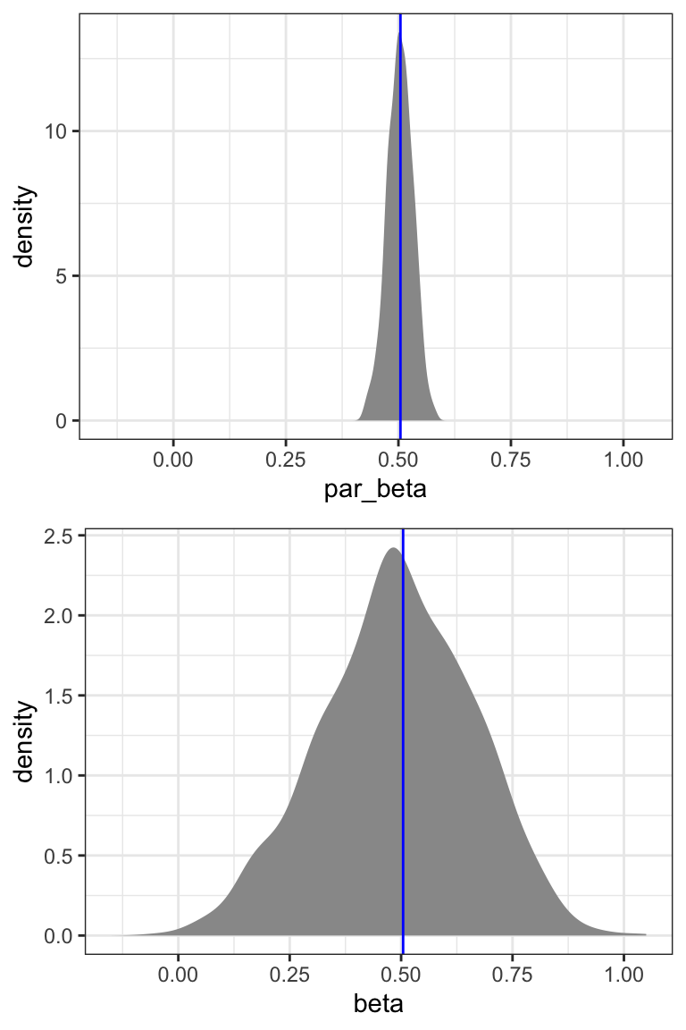 

Figure 13.1: Parametric (top) and nonparametric (bottom) bootstrap distributions of \(\hat{\beta}_{\mathrm{ad1}}\) using the Poisson model.

We observe that the standard error based on parametric bootstrapping is almost identical to the model based analytic estimate of the standard error. This suggests that if the data were from a Poisson model, the model based estimate would, in fact, be quite accurate. The standard error based on nonparametric bootstrapping is, however, around six times larger. This is in accordance with our previous observations that the Poisson model does not fit the data.

A standard confidence interval can be computed based on the nonparametric bootstrap estimate of the standard error, see Table 13.4. Alternatively, we can compute a confidence interval based on the simple combinant statistic \[ R(\hat{\beta}_{\mathrm{ad1}}, \beta_{\mathrm{ad1}}) = \hat{\beta}_{\mathrm{ad1}} - \beta_{\mathrm{ad1}}. \] Its distribution is approximated by the bootstrap distribution of \[ R(\hat{\beta}_{\mathrm{ad1}}^*, \hat{\beta}_{\mathrm{ad1}}) = \hat{\beta}_{\mathrm{ad1}}^* - \hat{\beta}_{\mathrm{ad1}}, \] where \(\hat{\beta}_{\mathrm{ad1}}^*\) denotes the parameter estimate for the nonparametrically bootstrapped sample. With \(\hat{w}_{\alpha}\) and \(\hat{z}_{\alpha}\) denoting the \(\alpha / 2\) and \(1 - \alpha / 2\) quantiles of the empirical bootstrap distribution of \(\hat{\beta}_{\mathrm{ad1}}^* - \hat{\beta}_{\mathrm{ad1}}\), we compute the confidence interval as \[ \{\beta \in \mathbb{R} \mid \hat{\beta}_{\mathrm{ad1}} - \beta \in (\hat{w}_{\alpha}, \hat{z}_{\alpha}) \} = (\hat{\beta}_{\mathrm{ad1}} - \hat{z}_{\alpha}, \hat{\beta}_{\mathrm{ad1}} - \hat{w}_{\alpha}). \] Note how it is the smaller quantile that determines the upper limit of the interval and the larger quantile that determines the lower limit. This results in the following confidence interval with nominal coverage 95%.

beta_star <- beta - boot_stat$beta_hat[1]
beta_qt <- quantile(beta_star, probs = c(0.975, 0.025), type = 1)
boot_stat$beta_hat[1] - beta_qt

    97.5%      2.5% 
0.2057629 0.8544931 

We can also bootstrap the distribution of the estimator based on the gamma model.

beta <- numeric(B)
for(b in 1:B) {
    i <- sample(n, n, replace = TRUE)  
    boot_glm <- glm(form, family = Gamma("log"), data = vegetables[i, ])
    beta[b] <- coefficients(boot_glm)["ad1"]
}

Figure 13.2: Nonparametric bootstrap distribution of \(\hat{\beta}_{\mathrm{ad1}}\) using the Gamma model.

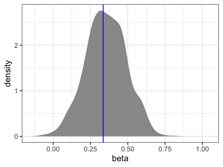
We will only consider the nonparametric bootstrap distribution for the gamma model as shown in Figure 13.2. We note that this distribution is closer to zero and also a bit narrower than the nonparametric bootstrap distribution based on the Poisson model.

All four nonparametric bootstrap intervals are in Table 13.4. The gamma model results in slightly narrower intervals than the Poisson model, and in intervals that are also closer to zero. There are small differences between the standard intervals and the simple intervals. This is most pronounced for the Poisson model, where the simple interval is moved slightly to the right relative to the standard interval. This corresponds to a slight left skewness in the bootstrapped distribution, see Figure 13.1.

interval	lower	upper
Gamma boot simple	0.06095	0.59121
Gamma boot se	0.06963	0.60059
Pois boot simple	0.20576	0.85449
Pois boot se	0.17139	0.83752

Table 13.4: The four bootstrap confidence intervals with nominal coverage 95%.

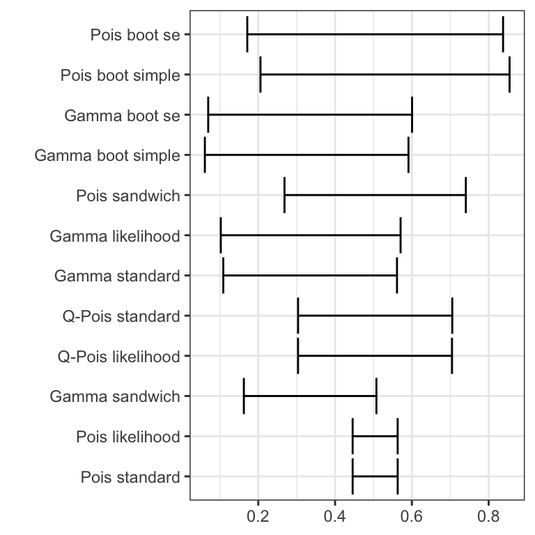
Figure 13.3 compares all twelve intervals computed using the two different models for estimation and using interval estimators that are either model based, robust or bootstrap based. The intervals are quite different, and this example shows first of all that statistical inference based on a misspecified model (the Poisson model) can be quite misleading. We make the following additional observations.

• The nonparametric bootstrap intervals are generally the widest intervals. Using the gamma model standard errors or the robust sandwich estimator for the Poisson model is a huge improvement over the Poison model based standard errors, but the nonparametric bootstrap suggests even wider intervals.
• The parametric bootstrap does not adjust for model misspecification and it usually gives intervals close to standard intervals using model based standard errors. It can be useful if we don’t have an analytic estimator of the standard error though.
• The gamma model and the Poisson model specify the same mean value model but result in different estimators (because they specify different variance models and thus different weights). Thus the estimates are different. If the gamma variance fits the data the best, the resulting estimator will also be more efficient. The same interval estimator gives narrower intervals for the gamma model estimator than for the Poisson model estimator,
  which suggest that the gamma model estimator is the most efficient.
• Irrespectively of which interval estimator we consider, the conclusion is still that there is a significant positive association between advertising and sale. But the evidence appears less strong and the magnitude much more undercertain than if we went with the initial conclusion based on the Poisson model only.

Figure 13.3: The twelve confidence intervals with nominal coverage 95% ordered according to width.

Using the nonparametric bootstrap to calibrate intervals to have the desired coverage usually performs quite well in practice for many estimators and for sufficiently large sample sizes. It is possible in special cases, or by relying on strong model assumptions, to analytically construct intervals with better coverage properties for small samples, but for moderate to large sample sizes the nonparametric bootstrap is hard to beat.

The main drawback of the bootstrap is a non-significant extra computational burden, since we need to refit the model \(B\) times. Though this computational cost scales linearly, it still means that if \(B = 999\) as above, and if it takes just one minute to compute the estimator for one dataset, it will take more than half a day to compute the bootstrap distribution. Since the bootstrap computations are embarrassingly parallel, the cost can partly be alleviated with access to many computational cores. However, such access appears to trigger the use of computationally more costly estimators in practice, and the bootstrap \(B\)-factor on the computational cost remains a challenge. This means that computationally cheaper alternatives are always of interest, and that we might want to save the computational costs until we are fairly sure about what we really want to bootstrap.

We could, of course, also always lower \(B\) to save some computations. As a rule of thumb, a choice of \(B = 200\) is actually sufficient if we just want an estimate of the standard error. The choice of \(B = 999\) as above is recommended for the estimation of 2.5% and 97.5% quantiles of any combinant statistic. If we want to estimate even more extreme quantiles with any accuracy we need \(B\) to be even larger.

Exercises

Exercise 13.1 Assume that the sample space is \(\mathbb{R}^k\) and the parameter of interest is the mean \[ \gamma(\rho) = \int y \, \mathrm{d}\rho(y). \] Assume that we have observations \(Y_1, \ldots, Y_n\) and let \(K\) denote the convex hull spanned by these observations (the smallest convex subset containing the observations). Let \(\hat{\rho}\) be the NPMLE, for which \[ \gamma(\hat{\rho}) = \frac{1}{n} Y_i. \]

1. Argue that if the support of \(\rho'\) is contained in \(K\) then \(\gamma(\rho') \in K\), and show that in this case there exists a \[ \rho = \sum_{i=1}^n \rho_i \varepsilon_{Y_i}. \] such that \(L(\rho) \geq L(\rho')\) and \(\gamma(\rho) = \gamma(\rho')\).

2. Show that if the support of \(\rho'\) is not restricted then for all \(\gamma \in \mathbb{R}^k\) \[ \sup_{\rho': \gamma(\rho') = \gamma} L(\rho') = L(\hat{\rho}). \]

Exercise 13.2 The Gompertz distribution on \([0, \infty)\) has survival function \[S (t) = \exp(- \eta (e^{\gamma t} - 1)) \quad t \geq 0, \] for parameters \(\eta, \gamma > 0\). We assume in the following that \[ (T_1, \delta_1), \ldots, (T_n, \delta_n) \] are \(n\) censored i.i.d. survival times following a Gompertz distribution. Introduce also the summary statistics \[ t = \sum_{i=1}^n T_i, \quad s = \sum_{i=1}^n \delta_i T_i \quad \textrm{and} \quad n_u = \sum_{i=1}^n \delta_i. \] The values of these summary statistics for a dataset are given in the following table together with some additional statistics.

Statistic:	\(n\)	\(n_u\)	\(t\)	\(s\)	\(\hat{\gamma}\)	\(\sum_{i=1}^n e^{\hat{\gamma} T_i}\)	\(\sum_{i=1}^n T_i^2 e^{\hat{\gamma} T_i}\)
Value:	50	32	1637	1384	0.09390	3396	9949983

1. Compute the hazard function for the Gompertz distribution. Show that the log-likelihood is \[ \ell(\eta, \gamma) = \log(\eta \gamma) n_u + \gamma s + \eta\left(n - \sum_{i=1}^n e^{\gamma T_i}\right). \]

2. Show that the MLE (provided it exists) satisfies the equations \[ \begin{align*} \sum_{i=1}^n e^{\gamma T_i} & = n + \frac{n_u}{\eta} \\ \sum_{i=1}^n T_i e^{\gamma T_i} & = \frac{s}{\eta} + \frac{n_u}{\eta \gamma}. \end{align*} \]

3. With \(\mathcal{J}^{\mathrm{obs}}\) denoting the observed Fisher information show that
   \[ ((\mathcal{J}^{\mathrm{obs}})^{-1})_{22} = \left(\frac{n_u}{\hat{\gamma}^2} + \hat{\eta} \sum_{i=1}^n T_i^2 e^{\hat{\gamma} T_i} - \frac{1}{n_u} \left(s + \frac{n_u}{\hat{\gamma}}\right)^2\right)^{-1}. \]

4. Using the summary statistics from the table above show that
   \[ \hat{\eta} = 0.009564 \] and compute an approximate likelihood interval for \(\gamma\).

From hereon it is assumed that the censoring distribution is exponential with rate parameter \(\lambda\), and that the censoring variables are i.i.d.

5. Argue why \(\hat{\lambda} = (n - n_u) / t\) is a sensible estimator of \(\lambda\).

6. Simulate a new data set, \((\tilde{T}_1, \tilde{\delta}_1), \ldots, (\tilde{T}_n, \tilde{\delta}_n)\), using the estimated parameters \(\hat{\eta}\) and \(\hat{\gamma}\) for the Gompertz survival distribution and \(\hat{\lambda}\) for the exponential censoring distribution. Compute and plot the Kaplan-Meier estimator of the survival function for the simulated data and compare it to the theoretical survival function.

The implementation of the simulation is the first step in the construction of a parametric bootstrap algorithm, which, for instance, can be used to calibrate the likelihood interval.

7. Implement a parametric bootstrap algorithm¹⁹ to obtain a bootstrap approximation of the distribution of the statistic \[ \frac{(\gamma - \hat{\gamma})^2}{((\mathcal{J}^{\mathrm{obs}})^{-1})_{22}}. \] Compare it with a \(\chi^2_1\)-distribution.

¹⁹ Remember the parameter constraints!

Hint: The implementation will require the numerical solution of the score equation for the computation of the MLE. You will only need to numerically solve a univariate equation, and you can implement your own Newton algorithm. You can also use the R function uniroot(). Alternatively, you can use the R function optim() for direct minimization of the negative log-likelihood.

Exercise 13.3 This exercise is investigating the effect of model selection on the standard confidence interval constructions.

The exercise uses the cholost data set from the R package RwR, and you will consider models of the effect of compliance on cholesterol decrease. Data is from a trial where 164 men took cholestyramine for a number of years. Their decrease in blood-level cholesterol from the beginning to the end of the trial is the response variable (y in the data set). Not all of them took the intended dose. In the data set the variable c measures compliance. It is a monotone transformation of the proportion of the dose actually taken.

The conditional expectation of the decrease in cholesterol level \(Y\) as a function of the compliance \(C\) is denoted \[ E(Y \mid C) = f(C), \] and it is assumed throughout that \(V(Y \mid C) = \sigma^2\).

1. Fit the model \[ f(c) = \beta_0 + \beta_1 c \] of the cholesterol decrease as a function of compliance. Investigate the model fit²⁰.

²⁰ This is a small data set, so don’t use hexagonal binning for plotting the data points!

In the following \(f\) is expanded using natural cubic splines. Using the R terminology, an expansion with \(\mathrm{df}\) degrees of freedom is a model with \(\mathrm{df} - 1\) knots, \(\mathrm{df}\) basis functions and \(\mathrm{df} + 1\) parameters (an intercept and one parameter for each of the basis functions).

2. Fit \(f\) as a natural cubic spline with 3 degrees of freedom. Give a graphical presentation of the resulting model. Compare the model to the linear regression model above.

3. In the remaining part of the exercise the focus is on the estimation of \(f(c)\) for \[ c \in I := \{-2, -1, 0, 1, 2\}. \] That is, the focus is on the computation of the estimators \(\hat{f}(c)\) and their distribution for \(c\) taking these five particular values.

4. Use nonparametric bootstrapping to estimate standard errors of \(\hat{f}(c)\) for \(c \in I\) when fitting the natural cubic spline model with 3 degrees of freedom. Compare with the theoretical values of the standard errors.

5. Consider the 6 models where \(f\) is a natural cubic spline with 1–6 degrees of freedom. Compare the models and use the adjusted \(R^2\)-statistic to select one of the 6 models.

The bootstrap above does not take into account any model selection such as the selection of degrees of freedom of the cubic spline expansion of \(f\). The last question in this problem explores the effect of model selection on the confidence intervals.

6. Use nonparametric bootstrapping to estimate standard errors of \(\hat{f}(c)\) for \(c \in I\) when selection of the degrees of freedom in the range from 1 to 6 is part of the estimation procedure. Compare with the previously estimated standard errors.

Exercise 13.4 Let \(\mathcal{L}(c)\) denote the likelihood regions from Definition 13.4.

1. Show that the MLE exists if and only if \(\bigcap_{c > 0} \mathcal{L}(c) \not = \emptyset\)
2. Show that the MLE is unique if and only if \(\bigcap_{c > 0} \mathcal{L}(c)\) is a singleton set.