library(RwR)
library(ggplot2)
library(tibble)
library(broom)
library(splines)2 The linear model
Warning
This chapter is still a draft and minor changes are made without notice.
The linear model is the classical workhorse of regression modeling. It is a tractable model with many desirable practical and theoretical properties. In combination with nonlinear variable transformations and basis expansions it can be surprisingly flexible, and even if it is not the optimal model choice in a given situation, it can work well as a benchmark or fallback model whenever more sophisticated models are considered.
2.1 Outline and prerequisites
This chapter introduces the linear model as well as aspects of the general regression modeling framework and terminology used throughout book. An example on fire insurance claim size modeling is introduced in Section 2.2 and used throughout the chapter to illustrate the theory. Section 2.5 covers how the linear model is fitted to data, and Section 2.6 gives results on the sampling distributions of parameter estimators and test statistics that are used in relation to the linear model. Section 2.7 and Section 2.8 treat model assessment and comparison using the claim size models to illustrate the theory. The chapter concludes in Section 2.9 by introducing basis expansion techniques to capture nonlinear relations within the framework of the linear model. The techniques are illustrated by a spline basis expansion of the relation between claim size and insurance sum in the fire insurance example.
The chapter primarily relies on the following four R packages.
A few functions from additional packages are used, but in those cases the package is made explicit via the :: operator.
2.2 Claim sizes
In this section we take a first look at a dataset from a Danish insurance company with the purpose of studying the relation between the insurance sum and the claim size for commercial fire claims. The data is included as the claims dataset in the RwR package.
data(claims, package = "RwR")We will use this dataset to build simple linear regression models that can predict potential claim sizes given knowledge of the insurance sums. More refined predictions as well as the possibility to differentiate policy prices can also be achieved by breaking down such a relation according to other variables.
tibble(claims) |> head()# A tibble: 6 × 3
claims sum grp
<dbl> <dbl> <fct>
1 3853. 34570294. 1
2 1194. 7776469. 1
3 3917. 26343305. 1
4 1259. 5502915. 1
5 11594. 711453346. 1
6 33535. 716609368. 1 To inspect the data we can print out a small part of the dataset using the head() function. There is a similar tail() function that prints the last part of the dataset.
The first column printed shows the row names (in this case just the row numbers). The other columns show the values of the variables in the date set. In this case the dataset contains the following three variables:
claims: the claim size in Danish kroners (DKK)sum: the insurance sum in Danish kroners (DKK)grp: the trade group of the business
The claims and sum variables are numeric, while the grp variable is a categorical trade group. The trade group is represented by integers but encoded and stored as a factor. The trade group encoding is:
- 1 = residences
- 2 = ordinary industry
- 3 = hotel and restaurant
- 4 = production industry
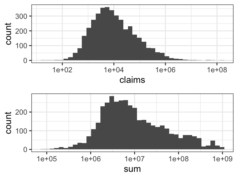
The marginal distributions of claim size and insurance sum are both highly skewed and span several orders of magnitude – as is revealed by the histograms in Figure 2.1. For this reason we will log-transform both variables in the subsequent figures. In this section this is purely for the purpose of better visualization. In later sections we will consider regression models for the log-transformed variables as well. Skewness of the marginal distributions does not automatically imply that the variables should be log-transformed for the regression model, and we will return to this discussion later.
Throughout we will avoid constructing new variables in the dataset that represent transformations of other variables. We will instead use the functionalities in R for changing the scale in a plot or for transforming one or more variables directly when fitting a model. The scatter plot in Figure 2.2 of claim size against insurance sum on a log-log-scale was constructed using ggplot() from the R package ggplot2.
Code
p0 <- ggplot(
        data = claims,
        aes(sum, claims),
        alpha = I(0.2)
    ) +
    scale_x_log10(
        "Insurance sum (DKK)",
        breaks = 10^c(6, 7, 8),
        labels = c("1M", "10M", "100M")
        ) +
    scale_y_log10(
        "Claim size (DKK)",
        breaks = 10^c(2, 4, 6, 8),
        labels = c("100", "10K", "1M", "100M")
    ) +
    geom_point()

p <- p0 +
    geom_smooth(
        method = "lm",
        linewidth = 1,
        se = FALSE
    )
p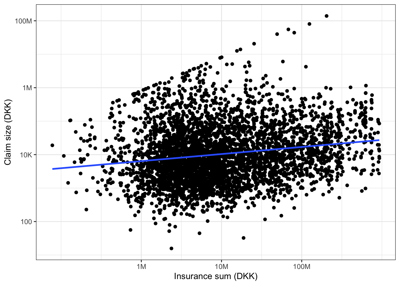
The code used to generate the plot shows that the plot is first stored as an R object named p and then plotted by “printing” p (the line just containing p). This is useful for later reuse of the same plot with some modifications as will be illustrated below. Note that the regression line was added to the plot using the geom_smooth() function with method = "lm".
From Figure 2.2 it appears that there is a positive correlation between the insurance sum and the claim size – the larger the insurance sum is, the larger is the claim size. Note the “line-up” of the extreme claim sizes, which (approximately) fall on the line with slope 1 and intercept 0. These claims are capped at the insurance sum, and we should pay some attention to the effect of these extremes in subsequent modeling steps.
The questions that we will focus on in this chapter are whether the trade group should be included into the model and whether a linear relation (on the log-log-scale) between the claim size and insurance sum is appropriate. As a first attempt to address the first question we stratify the scatter plot according to the trade group.
Code
p + facet_wrap(~ grp, ncol = 4)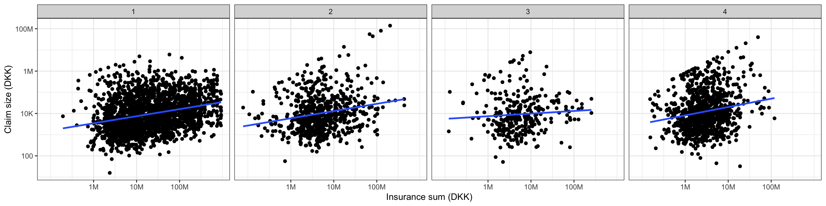
Figure 2.3 shows that there might be some differences, but it is difficult to tell from the figure alone if these differences are due to random variation or if they actually represent real differences between the groups.
The following sections will introduce the mathematical framework for fitting linear regression models and for investigating the models. Based on this theory we can tell if the model is an adequate model of the data and answer the questions put forward.
2.3 The linear model assumptions
This section briefly introduces the linear model and the typical assumptions made. This settles notation for the case study in the following section. In a first reading it can be read quickly and returned to later to better digest the model assumptions and their implications.
The linear model relates a continuous response variable \(Y\) to a \(p\)-dimensional vector \(X\) of predictors via the identity \[ E(Y \mid X) = X^T \beta. \tag{2.1}\] Here \[ X^T \beta = X_1 \beta_1 + \ldots + X_p \beta_p \] is a linear combination of the predictors weighted by the \(\beta\)-parameters and \(E(Y \mid X)\) denotes the conditional expectation of \(Y\) given \(X\). Thus the linear model is a model of the conditional expectation of the response variable given the predictors.
The entries of \(X\) go by many other names: explanatory variables, covariates, independent variables, regressors, inputs or features. Similarly, \(Y\) is also called the outcome or dependent variable.
An intercept parameter, \(\beta_0\), is often added, \[ E(Y \mid X) = \beta_0 + X^T \beta. \] It is notationally convenient to assume that the intercept parameter is included among the other parameters. This can be achieved by joining the predictor \(X_0 = 1\) to \(X\), thereby increasing the dimension to \(p + 1\). In the general presentation we will not pay particular attention to the intercept. We will assume that if an intercept is needed, it is appropriately included among the other parameters, and we will index the predictors from \(1\) to \(p\). Other choices of index set, e.g., from \(0\) to \(p\), may be convenient in specific cases.
In addition to the fundamental linearity expressed by Equation 2.1 we will for various reasons need additional model assumptions. For later reference we collect three standard model assumptions here.
A1. The conditional expectation of \(Y\) given \(X\) is \[E(Y \mid X) = X^T \beta.\]
Assumption A2 is sometimes called homoskedasticity, which is derived from the Greek words “homo” (same) and “skedastios” (dispersion). A violation of A2 is heteroskedasticity. Less pretentiously, we may call A2 variance homogeneity and refer to violations of A2 as variance inhomogeneity.
A2. The conditional variance of \(Y\) given \(X\) does not depend upon \(X\), \[V(Y \mid X) = \sigma^2.\]
A3. The conditional distribution of \(Y\) given \(X\) is a normal distribution, \[Y \mid X \sim \mathcal{N}(X^T\beta, \sigma^2).\]
It is, of course, implicit in A1 and A2 that \(Y\) has finite expectation and variance, respectively. It may not be obvious what the purpose of is. For once, it makes interpretations of the model and the assessment of the accuracy of model predictions easier, because it entails that the predictors primarily affect the response distribution via a location transform while the spread of the distribution is unaffected. Assumption A2 has, moreover, several consequences for the more technical aspect of the statistical analysis.
Assumption A3 is a strong distributional assumption, which entails A1 and A2 but is often unnecessarily restrictive for many purposes. Often A1 and A2 is sufficient, but whether A3 holds can be important when using the model to make probabilistic predictions, e.g., when computing prediction intervals. It is, in addition, only under Assumption A3 that an exact statistical theory can be developed for finite sample sizes. Some results used in practice are formally derived under this assumption, and they must be regarded as approximations when A3 is violated.
There exists a bewildering amount of terminology related to the linear model in the literature. Notation and terminology has been developed differently for different submodels of the linear model. If the \(X\)-vector only represents continuous variables, the model is often referred to as the linear regression model. Since any categorical variable can be encoded via \(k\) binary dummy variables (also known as a one-hot encoding), the linear model includes all ANalysis Of VAriance (ANOVA) models. Combinations, known in parts of the literature as ANalysis of COVAriance (ANCOVA), are of course also possible.
Dummy variable encoding: A categorical variable on \(k\) levels is encoded as a \(k\)-dimensional binary vector, whose \(j\)-th dummy variable equals \(1\) if the value of the categorical variable equals the \(j\)-th level and \(0\) otherwise.
Treating each special case separately and using special terminology is unnecessary and confusing – and most likely a consequence of historically different needs in different areas of applications. We give a unified treatment of the linear model. It is a fairly simple model with a rather complete theoretical basis. That said, many modeling questions still have to be settled for any specific real data analysis, which makes applications of even the simple linear model non-trivial.
For statistical applications we have a sample of \(n\) observations and to develop the statistical theory we need additional distributional assumptions regarding their joint distribution. Letting \(Y_1, \ldots, Y_n\) denote the \(n\) observations of the response with corresponding predictors \(X_1, \ldots, X_n\), we collect the responses into a column vector \(\mathbf{Y}\), and we collect the predictors into an \(n \times p\) matrix \(\mathbf{X}\) called the model matrix. The \(i\)-th row of \(\mathbf{X}\) is \(X_i^T\). The additional assumptions are:
The response vector and model matrix: \[
\mathbf{Y} = \left( \begin{array}{c} Y_1 \\ Y_2 \\ \vdots \\ Y_n \end{array} \right)
\qquad
\mathbf{X} = \left( \begin{array}{c} X_1^T \\ X_2^T \\ \vdots \\ X_n^T \end{array} \right)
\]
A4: The conditional distribution of \(Y_i\) given \(\mathbf{X}\) depends upon \(X_i\) only, and \(Y_i\) and \(Y_j\) are conditionally uncorrelated given \(\mathbf{X}\), \[\text{cov}(Y_i, Y_j \mid \mathbf{X}) = 0.\]
A5: The conditional distribution of \(Y_i\) given \(\mathbf{X}\) depends upon \(X_i\) only, and \(Y_1, \ldots, Y_n\) are conditionally independent given \(\mathbf{X}.\)
A6: The pairs \((X_1, Y_1), \ldots, (X_n, Y_n)\) are i.i.d.
There is a hierarchy among these three assumptions with A6 implying A5 and A5 implying A4. Thus A4 is the weakest distributional assumption about the joint distribution of the observations.
Assumption A4 implies together with A1 and A2 that \[ E(\mathbf{Y} \mid \mathbf{X}) = \mathbf{X} \beta, \tag{2.2}\] and that \[ V(\mathbf{Y} \mid \mathbf{X}) = \sigma^2 \mathbf{I} \tag{2.3}\] where \(\mathbf{I}\) denotes the \(n \times n\) identity matrix.
Assumptions A5 and A3 imply that \[ \mathbf{Y} \mid \mathbf{X} \sim \mathcal{N}(\mathbf{X}\beta, \sigma^2 \mathbf{I}). \tag{2.4}\] In summary, there are essentially two sets of distributional assumptions. The weak set A1, A2 and A4, which imply the moment identities (2.2) and (2.3), and the strong set A3 and A5, which, in addition, imply the distributional identity (2.4). Occasionally, A6 combined with A1 and A2 is used to justify certain resampling based procedures, such as bootstrapping, or to give asymptotic justifications of inference methodologies.
The linear regression model and the different assumptions related to it can also be phrased in terms of an additive error. The equation \[Y = X^T \beta + \epsilon.\] defines \(\epsilon\) – known as the error or noise term. In terms of \(\epsilon\) the model assumptions are as follows:
Definition of the additive error.
- A1 is equivalent to \(E(\epsilon \mid X) = 0\)
- A2 is equivalent to \(V(\epsilon \mid X) = \sigma^2\)
- A3 is equivalent to \(\epsilon \mid X \sim \mathcal{N}(0, \sigma^2)\).
Note that under Assumption A3, the conditional distribution of \(\epsilon\) given \(X\) does not depend upon \(X\), thus A3 implies that \(\epsilon\) and \(X\) are independent.
It is important to realize that the model assumptions cannot be justified prior to the data analysis. There are no magic arguments or simple statistical summaries that imply that the assumptions are fulfilled. A histogram of the marginal distribution of the responses can, for instance, not be used as an argument for or against Assumption A3 on the conditional normal distribution of \(Y\). Justifications and investigations of model assumptions are done after a model has been fitted to data. This is called model diagnostics.
2.4 Linear models of claim sizes
Returning to the insurance claim sizes, a regression model of log claim size, \(\log(Y_i)\), for insured \(i\) using log insurance sum, \(\log(X_{i, \texttt{sum}})\), as predictor can be fitted to data using the R function lm(). The theory behind the computations is treated in the subsequent section.
Code
claims_lm <- lm(
    log(claims) ~ log(sum),
    data = claims
)
coefficients(claims_lm)
(Intercept) log(sum)
5.8410060 0.2114886 This model is the linear model \[E(\log(Y_i) \mid X_{i, \texttt{sum}}) = \beta_0 + \beta_{\texttt{sum}} \log(X_{i, \texttt{sum}}).\] In the R terminology the parameter \(\beta_0\) is the (Intercept) coefficient and \(\beta_{\texttt{sum}}\) is the log(sum) coefficient. The model corresponds to the regression line shown in Figure 2.2.
Note that in concrete cases we will not write the conditioning variable explicitly as \(\log(X_{i, \texttt{sum}})\). As long as the right hand side is a linear combination of transformations of the conditioning variables (and an intercept) this is a linear model. It would be bothersome to write out explicitly the vector of transformations on the left hand side. These are, however, computed explicitly by and stored in the model matrix \(\mathbf{X}\).
Code
model.matrix(claims_lm)[781:784, ] (Intercept) log(sum)
781 1 19.42274
782 1 14.63276
783 1 14.90718
784 1 15.24711In the general treatment of the linear model it is notationally beneficial to always condition explicitly on the model matrix or a row in the model matrix. Thus to have a smooth notation in the general theory as well as in the concrete examples we will have to live with this slight discrepancy in notation. This will usually not be a source of confusion once the nature of this discrepancy is understood clearly. The models treated below illustrate this point further.
We can condition on the trade group, \(\texttt{grp}_i\), as well and thus consider the model \[ \begin{aligned} E(\log(Y_i) \mid X_{i, \texttt{sum}}, \texttt{grp}_i) & = \beta_0 + \beta_{\texttt{sum}} \log(X_{i, \texttt{sum}}) \\ & \hskip -1cm + \beta_{\texttt{grp2}} X_{i, \texttt{grp2}} + \beta_{\texttt{grp3}} X_{i, \texttt{grp3}} + \beta_{\texttt{grp4}} X_{i, \texttt{grp4}}. \end{aligned} \] This model is known as the additive model. The dummy variable encoding of the categorical trade group is used, and since the model includes an intercept the dummy variable corresponding to the first group is removed. Otherwise the model would be overparametrized. The consequence is that the first group acts as a baseline, and that the parameters \(\beta_{\texttt{grp2}}\), \(\beta_{\texttt{grp3}}\) and \(\beta_{\texttt{grp4}}\) are the differences from the baseline. These differences are also known as contrasts. We see, for example, that \[ E(\log(Y_i) \mid X_{i, \texttt{sum}} = x, \texttt{grp}_i = 1) = \beta_0 + \beta_{\texttt{sum}} \log(x) \] and \[ E(\log(Y_i) \mid X_{i, \texttt{sum}} = x, \texttt{grp} = 2) = \beta_0 + \beta_{\texttt{sum}} \log(x) + \beta_{\texttt{grp2}}, \] thus the difference from the baseline trade group 1 to trade group 2 is \(\beta_{\texttt{grp2}}\).
We can again fit this model using lm() in R, which automatically determines the model parametrization (using defaults) and computes the model matrix.
Code
claims_lm_add <- lm(
    log(claims) ~ log(sum) + grp,
    data = claims
)
coefficients(claims_lm_add)
(Intercept) log(sum) grp2 grp3 grp4
3.5974043 0.3300459 0.5472730 0.4013465 0.9143058 Code
model.matrix(claims_lm_add)[781:784, ] (Intercept) log(sum) grp2 grp3 grp4
781 1 19.42274 0 0 0
782 1 14.63276 1 0 0
783 1 14.90718 0 0 1
784 1 15.24711 1 0 0Alternative parametrizations can be specified using the contrasts argument.
Code
claims_lm_add <- lm(
    log(claims) ~ log(sum) + grp,
    data = claims,
    contrasts = list(grp = "contr.sum")
)
coefficients(claims_lm_add)
(Intercept) log(sum) grp1 grp2 grp3
4.06313567 0.33004591 -0.46573135 0.08154169 -0.06438483 Code
model.matrix(claims_lm_add)[781:784, ] (Intercept) log(sum) grp1 grp2 grp3
781 1 19.42274 1 0 0
782 1 14.63276 0 1 0
783 1 14.90718 -1 -1 -1
784 1 15.24711 0 1 0The contr.sum contrast gives the parametrization \[
\begin{aligned}
E(\log(Y_i) \mid X_{i, \texttt{sum}}, \texttt{grp}_i) & = \beta_0 + \beta_{\texttt{sum}} \log(X_{i, \texttt{sum}}) \\
& + \beta_{\texttt{grp1}} X_{i, \texttt{grp1}} + \beta_{\texttt{grp2}} X_{i, \texttt{grp2}} \\
& + \beta_{\texttt{grp3}} X_{i, \texttt{grp3}} + \beta_{\texttt{grp4}} X_{i, \texttt{grp4}}.
\end{aligned}
\] with the constraint \(\beta_{\texttt{grp1}} + \beta_{\texttt{grp2}} + \beta_{\texttt{grp3}} + \beta_{\texttt{grp4}} = 0\). Only the parameters \(\beta_{\texttt{grp1}}\), \(\beta_{\texttt{grp2}}\) and \(\beta_{\texttt{grp3}}\) are reported, and \(\beta_{\texttt{grp4}} = - \beta_{\texttt{grp1}} - \beta_{\texttt{grp2}} - \beta_{\texttt{grp3}}\) as can also be seen from the model matrix. This latter parametrization can be more convenient if we want to compare trade groups to the overall intercept instead of to one specific baseline group.
The additive model gives a different intercept for each trade group but the slope is kept the same for all trade groups. Within the framework of linear models we can capture differences in slope as an interaction between the insurance sum and the trade group. Using the parametrization with trade group 1 as baseline this model is \[ \begin{aligned} E(\log(Y_i) \mid X_{i, \texttt{sum}}, \texttt{grp}_i) & = \beta_0 + \beta_{\texttt{sum}} \log(X_{i, \texttt{sum}}) \\ & + (\beta_{\texttt{grp2}} + \beta_{\texttt{sum}, \texttt{grp2}} \log(X_{i, \texttt{sum}}))X_{i, \texttt{grp2}} \\ & + (\beta_{\texttt{grp3}} + \beta_{\texttt{sum}, \texttt{grp3}} \log(X_{i, \texttt{sum}}))X_{i, \texttt{grp3}} \\ & + (\beta_{\texttt{grp4}} + \beta_{\texttt{sum}, \texttt{grp4}} \log(X_{i, \texttt{sum}}))X_{i, \texttt{grp4}}. \end{aligned} \]
The parameter estimates and model matrix are:
Code
coefficients(claims_lm_int) |> print(width = 120) (Intercept) log(sum) grp2 grp3 grp4 log(sum):grp2 log(sum):grp3 log(sum):grp4
3.525657166 0.334288387 0.434262343 3.666489986 0.040781595 0.007719206 -0.209986484 0.059341891 Code
model.matrix(claims_lm_int)[781:784, ] |> print(width = 120) (Intercept) log(sum) grp2 grp3 grp4 log(sum):grp2 log(sum):grp3 log(sum):grp4
781 1 19.42274 0 0 0 0.00000 0 0.00000
782 1 14.63276 1 0 0 14.63276 0 0.00000
783 1 14.90718 0 0 1 0.00000 0 14.90718
784 1 15.24711 1 0 0 15.24711 0 0.00000This model corresponds to the regression lines shown in Figure 2.3. This example illustrates why we do not want to write out the eight dimensional vector explicity in the condition when in fact it is just a transformation of \(X_{i, \texttt{sum}}\) and \(\texttt{grp}_i\). On the other hand, it would be equally bothersome to drag an abstract transformation around in the general notation.
Three linear models were considered in this section, and subsequent sections and chapters will treat different ways of comparing models and for drawing inference about model parameters and hypotheses. It must be emphasized that the purpose of developing the theory and the corresponding statistical methods is not to be able to deduce from data what the “true model” is. There are several reasons for that. For once, all models should be considered as approximations only. We can try to find an adequate model approximation that captures essential aspects of the data, and we may be able to justify that a model is adequate, but we will never be able to justify that a model is “true”.
All models are wrong but some are useful. George Box, 1978
Several models may also be valid and yet appear contradictory, and it may then depend on the purpose of the modeling which to use. It is, for instance, important to formulate precisely which predictors that we condition on. Suppose that the conditional expectation \(E(\log(Y_i) \mid X_{i, \texttt{sum}}, \texttt{grp}_i)\) is given by the additive model, say, then it follows from the tower property of conditional expectations that \[ \begin{aligned} E(\log(Y_i) \mid X_{i, \texttt{sum}}) & = \beta_0 + \beta_{\texttt{sum}} \log(X_{i, \texttt{sum}}) \\ & + \beta_{\texttt{grp2}} P(\texttt{grp}_i = 2 \mid X_{i, \texttt{sum}}) \\ & + \beta_{\texttt{grp3}} P(\texttt{grp}_i = 3 \mid X_{i, \texttt{sum}}) \\ & + \beta_{\texttt{grp4}} P(\texttt{grp}_i = 4 \mid X_{i, \texttt{sum}}). \end{aligned} \]
Now if \[ P(\texttt{grp}_i = k \mid X_{i, \texttt{sum}}) \approx \delta_k + \gamma_k \log(X_{i, \texttt{sum}}) \] for \(k = 2,3, 4\) then the linear model \[ E(\log(Y_i) \mid X_{i, \texttt{sum}}) = \beta_0 + \beta_{\texttt{sum}} \log(X_{i, \texttt{sum}}) \] will be an approximately valid model as well. However, the intercept and slope for this model may differ from the model where we condition also on the group. This depends on whether or not the \(\beta_{\texttt{grp}k}\), \(\delta_k\) and \(\gamma_k\) parameters are 0. If the \(\beta_{\texttt{grp}k}\) parameters were all 0 it would not matter if group is included in the conditioning. If group and insurance sum were independent then \(\gamma_k = 0\), and both models would be equally valid models of the conditional expectation of the log claim size. The slope would then be the same in both models but the intercept would differ. If group and insurance sum were dependent then the slope would depend on whether we condition on insurance sum only or whether we condition on insurance sum as well as group.
The approximation can be justified locally using Taylor’s theorem if the probability depends smoothly on the predictor.
The key take-home message is that a predictor variable may be excluded from the model even if it has a non-zero coefficient without necessarily invalidating the model. Another take-home message is that there is no such thing as an unqualified “effect” of a predictor variable. Effect sizes, as quantified by the \(\beta\) coefficients, are always depending upon exactly which variables we condition on, whether this is made explicit by the modeling or is implicit by the data sampling process.
In the light of George Box’s famous aphorism above it is only appropriate to give another Box quote: Since all models are wrong the scientist must be alert to what is importantly wrong (Box 1976). One place to start is to investigate the assumptions A1, A2 and A3. These are investigated after the model has been fitted to data typically via the residuals \[ \hat{\epsilon}_i = Y_i - X_i^T \hat{\beta} \tag{2.5}\] that are approximations of the errors \(\epsilon_i\).
Box, George E. P. 1976. “Science and Statistics.” Journal of the American Statistical Association 71 (356): 791–99.
Code
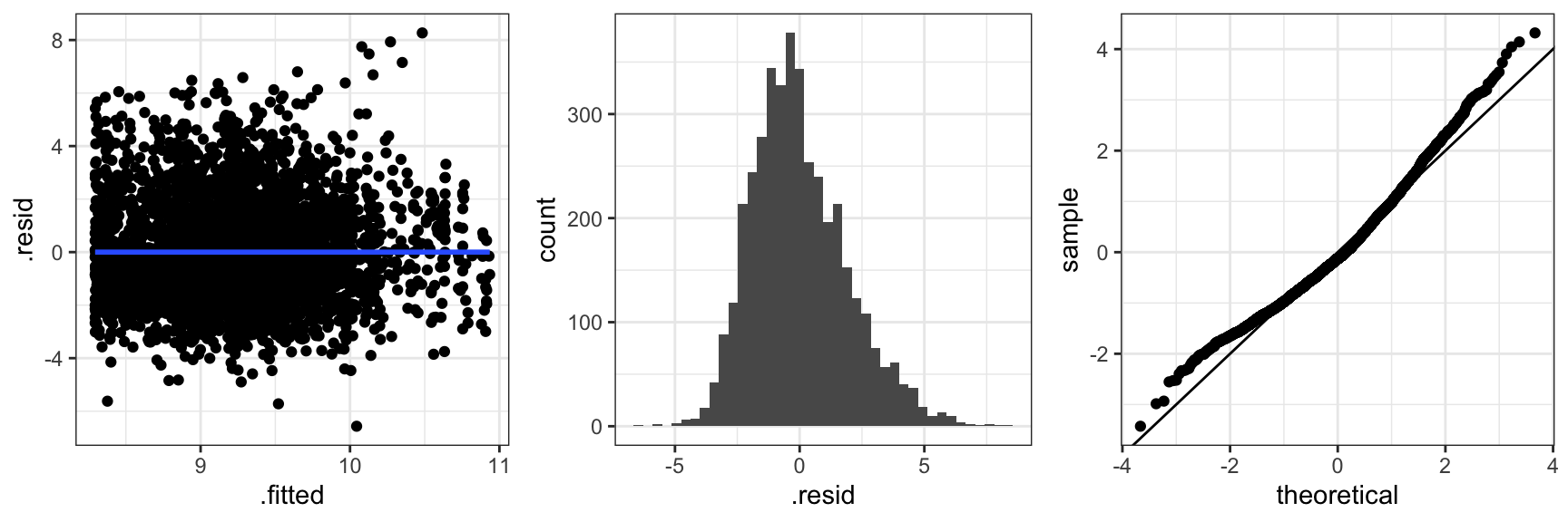
claims_diag <- augment(claims_lm) ## Residuals etc.
gridExtra::grid.arrange(
  ggplot(claims_diag, aes(.fitted, .resid), alpha = I(0.2)) + geom_point() + geom_smooth(),
  ggplot(claims_diag, aes(.resid)) + geom_histogram(bins = 40),
  ggplot(claims_diag, aes(sample = .std.resid)) + geom_qq() + geom_abline(),
  ncol = 3
)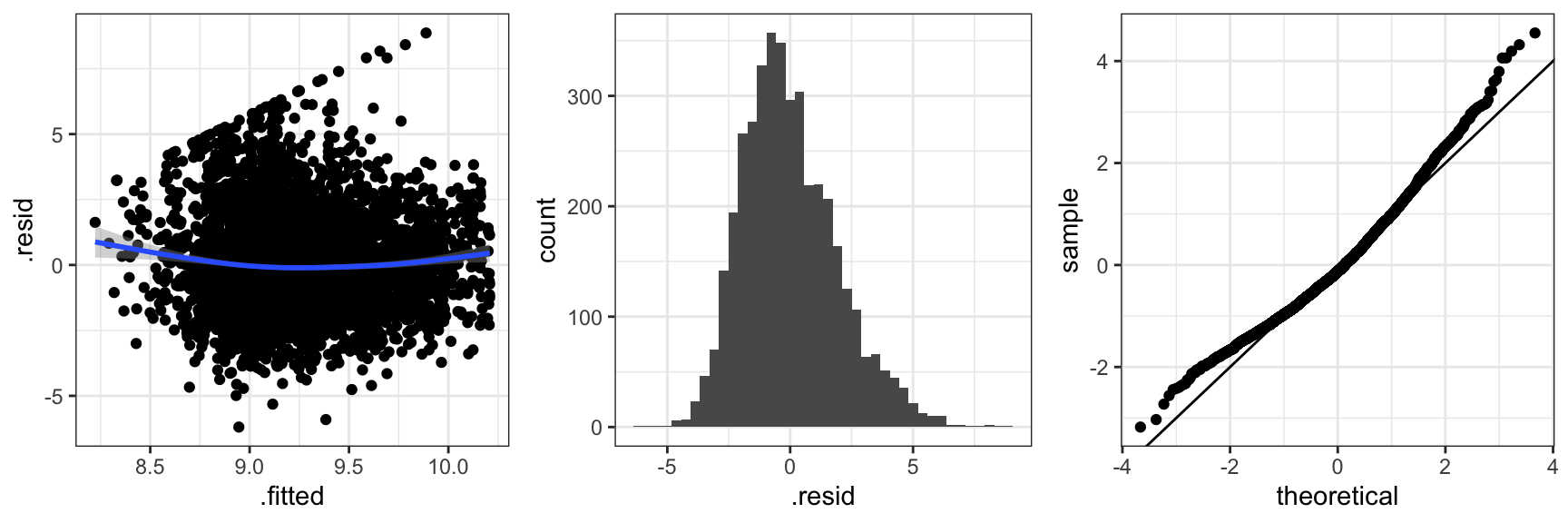
Figure 2.4 shows three typical diagnostic plots. The residuals plotted against the fitted values, \(X_i^T \hat{\beta}\), can be used to detect if the mean value specification is adequate and if the variance is approximately constant as a function of the fitted values. The scatter plot smoother added to the residual plot bends up in the ends indicating that the mean is not spot on. There is no clear indication of variance inhomogeneity. The histogram of the residuals and the qq-plot of the standardized residuals can be used for comparing the residual distribution with the normal distribution. In this case the residuals have a slightly right skewed distribution when compared to the normal distribution. Of course we also note the pattern of the most extreme positive residuals that correspond to the capped claims. In this section we will not pursue the effect of those.
Code
claims_diag_int <- augment(claims_lm_int) ## Residuals etc.
gridExtra::grid.arrange(
  ggplot(claims_diag_int, aes(.fitted, .resid), alpha = I(0.2)) + geom_point() + geom_smooth(),
  ggplot(claims_diag_int, aes(.resid)) + geom_histogram(bins = 40),
  ggplot(claims_diag_int, aes(sample = .std.resid)) + geom_qq() + geom_abline(),
  ncol = 3
)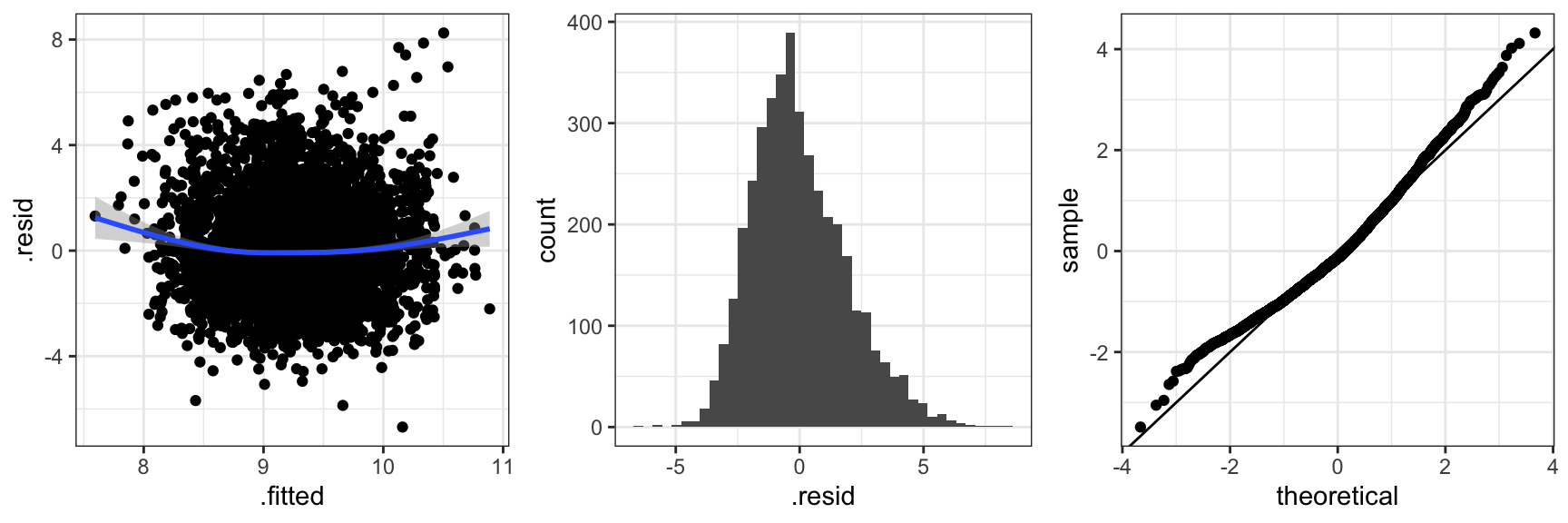
Figure 2.5 shows diagnostic plots for the more complicated interaction model. The conclusion is the same as for the simpler model. The mean value model is not spot on and the residual distribution is slightly skewed. This is not a bad model fit but it leaves room for improvements.
2.5 Estimation theory
The theory that we will cover in this section is on the estimation of the unknown parameter \(\beta\) using least squares methods. We give theoretical results on the existence and uniqueness, and we provide characterizations of the least squares estimator. We also discuss how the estimator is computed in practice.
2.5.1 Weighted linear least squares estimation
We will consider the generalization of linear least squares that among other things allows for weights on the individual cases. Allowing for weights can be of interest in itself, but serves, in particular, as a preparation for the methods we will consider in Chapter 6.
We introduce the weighted squared error loss as \[
\ell(\beta) = (\mathbf{Y} - \mathbf{X}\beta)^T\mathbf{W}(\mathbf{Y}
- \mathbf{X}\beta)
\tag{2.6}\] where \(\mathbf{W}\) is a positive definite matrix. An \(n \times n\) matrix is positive definite if it is symmetric and \[\mathbf{y}^T \mathbf{W} \mathbf{y} > 0\] for all \(\mathbf{y} \in \mathbb{R}^n\) with \(\mathbf{y} \neq 0\). A special type of positive definite weight matrix is a diagonal matrix with positive entries in the diagonal. With
\[
\mathbf{W} = \left(\begin{array}{cccc}
w_1 & 0 & \ldots & 0 \\
0 & w_2 & \ldots & 0 \\
\vdots & \vdots & \ddots & \vdots \\
0 & 0 & \ldots & w_n \end{array}\right)
\] we find that the weighted squared error loss becomes \[
\ell(\beta) = \sum_{i} w_i (Y_i - X_i^T \beta)^2.
\] That is, the \(i\)-th case receives the weight \(w_i\).
With \(\mathbf{W} = \mathbf{I}\) this loss is proportional to the negative log-likelihood loss under assumptions A3 and A5 as derived in Chapter 6.
We will estimate the parameter \(\beta\) via minimization of \(\ell\) – or via minimization of \(\ell\) plus a penalty term. With \(\boldsymbol{\Omega}\) a positive semidefinite \(p \times p\) matrix we will seek to minimize the function
\[
\ell_{\boldsymbol{\Omega}}(\beta) := \ell(\beta) + \beta^T \boldsymbol{\Omega} \beta.
\tag{2.7}\] The penalty term, \(\beta^T \boldsymbol{\Omega} \beta\), introduces a form of control on the minimization problem, and thus the estimator, by shrinking the minimizer toward 0. This can have beneficial numerical as well as statistical consequences. The purpose of introducing a penalty will be elaborated upon in subsequent sections, where some concrete examples will be given.
Equation 2.8 is called the normal equation.
Theorem 2.1 A solution to the equation \[ \left(\mathbf{X}^T \mathbf{W} \mathbf{X} + \boldsymbol{\Omega}\right) \beta = \mathbf{X}^T \mathbf{W} \mathbf{Y} \tag{2.8}\] is a minimizer of the quadratic loss function (2.7). There is a unique minimizer if either \(\mathbf{X}\) has full column rank \(p\) or if \(\boldsymbol{\Omega}\) is positive definite.
Proof. The derivative of \(\ell_{\boldsymbol{\Omega}}\) is \[ D_{\beta} \ell_{\boldsymbol{\Omega}}(\beta) = -2(\mathbf{Y} - \mathbf{X}\beta)^T \mathbf{W} \mathbf{X} + 2 \beta^T \boldsymbol{\Omega}. \]
To compute this derivative, it may be useful to think of \(\ell\) as a composition. The function \(a(\beta) = (\mathbf{Y} - \mathbf{X}\beta)\) from \(\mathbb{R}^{p}\) to \(\mathbb{R}^n\) has derivative \(D_{\beta}a(\beta) = -\mathbf{X}\), and \(\ell\) is a composition of \(a\) with the function \(b(z) = z^T \mathbf{W} z\) from \(\mathbb{R}^n\) to \(\mathbb{R}\) with derivative \(D_z b(z) = 2 z^T \mathbf{W}\). By the chain rule \[ D_{\beta} \ell(\beta) = D_zb(a(\beta)))D_{\beta}a(\beta) = -2(\mathbf{Y} - \mathbf{X}\beta)^T \mathbf{W} \mathbf{X}. \]
The derivative of \(\beta \mapsto \beta^T \boldsymbol{\Omega} \beta\) is found in the same way as the derivative of \(b\). Note that the derivative is a row vector.1
1 The gradient, \[\nabla_{\beta} \ell(\beta) = D_{\beta} \ell(\beta)^T,\] is a column vector.
We note that Equation 2.8 is equivalent to \(D_{\beta} \ell_{\boldsymbol{\Omega}}(\beta) = 0\), hence a solution of Equation 2.8 is a stationary point of \(\ell_{\boldsymbol{\Omega}}\).
The second derivative of \(\ell_{\boldsymbol{\Omega}}\) is \[ D_{\beta}^2 \ell_{\boldsymbol{\Omega}}(\beta) = 2 \left(\mathbf{X}^T \mathbf{W} \mathbf{X} + \boldsymbol{\Omega}\right). \] This matrix is (globally) positive semidefinite, hence the function is convex and any stationary point is a global minimum.
If \(\mathbf{X}\) has rank \(p\) or if \(\boldsymbol{\Omega}\) is positive definite, \(D_{\beta}^2 \ell_{\boldsymbol{\Omega}}(\beta)\) is positive definite and the minimizer of \(\ell_{\boldsymbol{\Omega}}\) is the unique solution of Equation 2.8.
When the solution to Equation 2.8 is unique it can, of course, be written as \[ \hat{\beta} = (\mathbf{X}^T \mathbf{W} \mathbf{X} + {\boldsymbol{\Omega}})^{-1} \mathbf{X}^T \mathbf{W} \mathbf{Y}. \] This can be a theoretically convenient formula for the estimator, but as we discuss below, the practical computation of \(\hat{\beta}\) does typically not rely on explicit matrix inversion.
A geometric interpretation of the weighted least squares estimator without penalization provides additional insights. The inner product induced by \(\mathbf{W}\) on \(\mathbb{R}^n\) is given by \(\mathbf{y}^T \mathbf{W} \mathbf{x}\), and the corresponding norm is denoted \(\|\cdot\|_{\mathbf{W}}\). With this notation we see that \[ \ell(\beta) = \|\mathbf{Y} - \mathbf{X}\beta\|^2_{\mathbf{W}}. \] If \(L = \{\mathbf{X}\beta \mid \beta \in \mathbb{R}^p\}\) denotes the column space of \(\mathbf{X}\), \(\ell\) is minimized whenever \(\mathbf{X}\beta\) is the orthogonal projection of \(\mathbf{Y}\) onto \(L\) in the inner product given by \(\mathbf{W}\).
In the rest of this section we only consider the case with \({\boldsymbol{\Omega}} = 0\).\(\|\mathbf{y}\|_{\mathbf{W}}^2 = \mathbf{y}^T \mathbf{W} \mathbf{y}\) specifies a norm if and only if \(\mathbf{W}\) is positive definite.
Lemma 2.1 The orthogonal projection onto \(L\) is \[ P = \mathbf{X} (\mathbf{X}^T \mathbf{W} \mathbf{X})^{-1} \mathbf{X}^T \mathbf{W} \] provided that \(\mathbf{X}\) has full column rank \(p\).
Proof. We verify that \(P\) is the orthogonal projection onto \(L\) by verifying three characterizing properties: \[ \begin{align*} P \mathbf{X} \beta & = \mathbf{X} \beta \quad (P \text{ is the identity on } L) \\ P^2 & = \mathbf{X} (\mathbf{X}^T \mathbf{W} \mathbf{X})^{-1} \mathbf{X}^T \mathbf{W} \mathbf{X} (\mathbf{X}^T \mathbf{W} \mathbf{X})^{-1} \mathbf{X}^T \mathbf{W} \\ & = \mathbf{X} (\mathbf{X}^T \mathbf{W} \mathbf{X})^{-1} \mathbf{X}^T \mathbf{W} = P \\ P^T \mathbf{W} & = (\mathbf{X} (\mathbf{X}^T \mathbf{W} \mathbf{X})^{-1} \mathbf{X}^T \mathbf{W} )^T \mathbf{W} \\ & = \mathbf{W} \mathbf{X} (\mathbf{X}^T \mathbf{W} \mathbf{X})^{-1} \mathbf{X}^T \mathbf{W} = \mathbf{W} P. \end{align*} \]
The last property is self-adjointness w.r.t. the inner product given by \(\mathbf{W}\).
Note that for \(\boldsymbol{\Omega} = 0\), Theorem 2.1 is a consequence of Lemma 2.1. This follows from the identity \(P\mathbf{Y} = \mathbf{X} \hat{\beta}\), since the equation \(P\mathbf{Y} = \mathbf{X} \beta\) has a unique solution when the columns of \(\mathbf{X}\) are linearly independent.
If \(\mathbf{X}\) does not have rank \(p\) the projection is still well defined, and it can be written as \[ P = \mathbf{X} (\mathbf{X}^T \mathbf{W} \mathbf{X})^{-} \mathbf{X}^T \mathbf{W} \] where \((\mathbf{X}^T \mathbf{W} \mathbf{X})^{-}\) denotes a generalized inverse. This is seen by verifying the same three conditions as in the proof above. The solution to \(P\mathbf{Y} = \mathbf{X} \beta\) is, however, no longer unique, and the solution \[ \hat{\beta} = (\mathbf{X}^T \mathbf{W} \mathbf{X})^{-} \mathbf{X}^T \mathbf{W} \mathbf{Y} \] is just one possible solution.
A generalized inverse of a matrix \(A\) is any matrix \(A^{-}\) with the property that \[AA^{-}A = A.\]
%% Moore-Penrose pseudoinverse and norm-minimal solutions.
2.5.2 Algorithms
The actual computation of the solution to the normal equation is typically based on a QR decomposition of \(\mathbf{X}\) and not on a matrix inversion or a direct solution of the linear equation. The R function lm() – or rather the underlying R functions lm.fit() and lm.wfit() – are based on the QR decomposition. We first treat the case \(\mathbf{W} = \mathbf{I}\) and \(\boldsymbol{\Omega} = 0\) and then subsequently the more general cases.
The normal equation can be solved by Gaussian elimination, which corresponds to an LU decomposition of \[\mathbf{X}^T \mathbf{W} \mathbf{X} + \boldsymbol{\Omega}.\] The algorithm was named after Carl Friedrich Gauss, though he did not invent it. However, he promoted it for efficient computation of the solution of least squares problems.
The QR decomposition of \(\mathbf{X}\) is the factorization \[
\mathbf{X} = \mathbf{Q} \mathbf{R},
\] where \(\mathbf{Q}\) is an orthogonal matrix and \(\mathbf{R}\) is an upper triangular matrix. Since \[
\mathbf{X}^T \mathbf{X} = \mathbf{R}^T \underbrace{\mathbf{Q}^T \mathbf{Q}}_{\mathbf{I}} \mathbf{R} = \mathbf{R}^T \mathbf{R},
\tag{2.9}\] the normal equation becomes \[
\mathbf{R}^T \mathbf{R} \beta = \mathbf{X}^T \mathbf{Y}.
\] This equation can be solved efficiently and in a numerically stable way in a two-step pass by exploiting first that \(\mathbf{R}^T\) is lower triangular and then that \(\mathbf{R}\) is upper triangular. Moreover, the QR decomposition can be implemented in a rank revealing way. This is useful when \(\mathbf{X}\) does not have rank \(p\), in which case the QR decomposition effectively reparametrizes the model as if some columns were removed from \(\mathbf{X}\). Such a version of the QR decomposition is used by lm.fit() and lm.wfit() in R, and one will obtain parameter estimates with the value NA when \(\mathbf{X}\) has (numerical) rank strictly less than \(p\).
For a general weight matrix we write \(\mathbf{W} = \mathbf{L} \mathbf{L}^T\), in which case the normal equation can be rewritten as \[ (\mathbf{L}^T \mathbf{X})^T \mathbf{L}^T \mathbf{X} \beta = (\mathbf{L}^T \mathbf{X})^T \mathbf{L}^T \mathbf{Y} \] Thus by replacing \(\mathbf{X}\) with \(\mathbf{L}^T \mathbf{X}\) and \(\mathbf{Y}\) with \(\mathbf{L}^T \mathbf{Y}\) we can proceed as above and solve the normal equation via a QR decomposition of \(\mathbf{L}^T\mathbf{X}\).
This could be the Cholesky decomposition with \(\mathbf{L}\) lower triangular, or \(\mathbf{L}\) could be the symmetric square root of \(\mathbf{W}\). For a diagonal \(\mathbf{W}\), \(\mathbf{L}\) is diagonal and trivial to compute by taking square roots. For unstructured \(\mathbf{W}\) the computation of the Cholesky decomposition scales as \(n^3\).
The computations based on the QR decomposition don’t involve the computation of the cross product \(\mathbf{X}^T \mathbf{X}\) (or more generally, \(\mathbf{X}^T \mathbf{W} \mathbf{X}\)). The factorization (2.9) of the positive semidefinite matrix \(\mathbf{X}^T \mathbf{X}\) as a lower and upper triangular matrix is called the Cholesky decomposition, and as outlined above it can be computed via the QR decomposition of \(\mathbf{X}\). An alternative is to compute \(\mathbf{X}^T \mathbf{X}\) directly and then compute its Cholesky decomposition. The QR decomposition is usually preferred for numerical stability. Computing \(\mathbf{X}^T \mathbf{X}\) is essentially a squaring operation, and precision can be lost. However, if \(n\) is large compared to \(p\) it will be faster to compute the Cholesky decomposition from the cross product.
If \(\boldsymbol{\Omega} \neq 0\) the normal equation can be solved by computing the Cholesky decomposition \[ \mathbf{X}^T \mathbf{W} \mathbf{X} + \boldsymbol{\Omega} = \mathbf{R}^T \mathbf{R} \] directly and then proceed as above.
To use the QR decomposition we write \(\boldsymbol{\Omega} = \mathbf{D} \mathbf{D}^T\). Then the normal equation can be written as \[ \left(\begin{array}{cc} \mathbf{X}^T \mathbf{L} & \mathbf{D} \end{array} \right) \left(\begin{array}{c} \mathbf{L}^T \mathbf{X} \\ \mathbf{D}^T \end{array} \right) \beta = \left(\begin{array}{cc} \mathbf{X}^T\mathbf{L} & \mathbf{D} \end{array} \right) \left(\begin{array}{c} \mathbf{L}^T \mathbf{Y} \\ 0 \end{array} \right). \] By replacing \(\mathbf{X}\) with \[ \left(\begin{array}{c} \mathbf{L}^T \mathbf{X} \\ \mathbf{D}^T \end{array} \right) \] and \(\mathbf{Y}\) with \[ \left(\begin{array}{c} \mathbf{L}^T \mathbf{Y} \\ 0 \end{array} \right) \] we can solve the normal equation via the QR decomposition as above.
The computations could again be done via the Cholesky decomposition of \(\boldsymbol{\Omega}\), or \(\mathbf{D}\) could be computed as the symmetric square root of \(\boldsymbol{\Omega}\).
2.6 Sampling distributions
In this section we give results on the distribution of the estimator, \(\hat{\beta}\), and test statistics of linear hypotheses under the weak assumptions A1, A2 and A4 and under the strong assumptions A3 and A5. Under the weak assumptions we can only obtain results on moments, while the strong distributional assumptions give exact sampling distributions. Throughout we restrict attention to the case where \(\mathbf{W} = \mathbf{I}\) and \(\boldsymbol{\Omega} = 0\).
2.6.1 Moments
Some results involve the unknown variance parameter \(\sigma^2\) (see Assumption A2) and some involve a specific estimator \(\hat{\sigma}^2\). This estimator of \(\sigma^2\) is \[ \hat{\sigma}^2 = \frac{1}{n-p} \sum_{i=1}^{n} (Y_i - X_i^T\hat{\beta})^2 = \frac{1}{n-p} \|\mathbf{Y} - \mathbf{X}\hat{\beta}\|^2 \tag{2.10}\] provided that \(\mathbf{X}\) has full rank \(p\). Recalling that the \(i\)-th residual is \[\hat{\epsilon}_i = Y_i - X_i^T\hat{\beta},\] the variance estimator equals the empirical variance of the residuals – up to division by \(n-p\) and not \(n\). Since the residual is a natural estimator of the unobserved error \(\epsilon_i\), the variance estimator \(\hat{\sigma}^2\) is a natural estimator of the error variance \(\sigma^2\). The explanation of the denominator \(n-p\) is related to the fact that \(\hat{\epsilon}_i\) is an estimator of \(\epsilon_i\). A partial justification, as shown in the following theorem, is that division by \(n-p\) makes \(\hat{\sigma}^2\) unbiased.
Theorem 2.2 Under the weak assumptions A1, A2 and A4, and assuming that \(\mathbf{X}\) has full rank \(p\), \[ \begin{align*} E(\hat{\beta} \mid \mathbf{X}) & = \beta, \\ V(\hat{\beta} \mid \mathbf{X}) & = \sigma^2 (\mathbf{X}^T\mathbf{X})^{-1}, \\ E(\hat{\sigma}^2 \mid \mathbf{X}) &= \sigma^2. \end{align*} \]
Proof. Using assumptions A1 and A4 we find that \[ \begin{align*} E(\hat{\beta} \mid \mathbf{X}) & = E((\mathbf{X}^T\mathbf{X})^{-1} \mathbf{X}^T \mathbf{Y} \mid \mathbf{X}) \\ & = (\mathbf{X}^T\mathbf{X})^{-1} \mathbf{X}^T E(\mathbf{Y} \mid \mathbf{X}) \\ & = (\mathbf{X}^T\mathbf{X})^{-1} \mathbf{X}^T \mathbf{X} \beta \\ & = \beta. \end{align*} \] Using assumptions A2 and A4 it follows that \[ \begin{align*} V(\hat{\beta} \mid \mathbf{X}) & = (\mathbf{X}^T\mathbf{X})^{-1} \mathbf{X}^T V(\mathbf{Y} \mid \mathbf{X}) \mathbf{X} (\mathbf{X}^T\mathbf{X})^{-1} \\ & = (\mathbf{X}^T\mathbf{X})^{-1} \mathbf{X}^T \sigma^2 \mathbf{I} \mathbf{X} (\mathbf{X}^T\mathbf{X})^{-1} \\ & = \sigma^2 (\mathbf{X}^T\mathbf{X})^{-1}. \end{align*} \]
For the computation of the expectation of \(\hat{\sigma}^2\), the geometric interpretation of \(\hat{\beta}\) is useful. Since \(\mathbf{X} \hat{\beta} = P \mathbf{Y}\) with \(P\) the orthogonal projection onto the column space \(L\) of \(\mathbf{X}\), we find that \[
\mathbf{Y} - \mathbf{X} \hat{\beta} = (\mathbf{I} - P) \mathbf{Y}.
\] Because \(E(\mathbf{Y} - \mathbf{X} \hat{\beta} \mid \mathbf{X}) = 0\) \[
E(\|\mathbf{Y} - \mathbf{X} \hat{\beta}\|^2 \mid \mathbf{X}) = \sum_{i=1}^n V(\mathbf{Y} - \mathbf{X} \hat{\beta} \mid \mathbf{X})_{ii}
\] and
\[
\begin{align*}
V(\mathbf{Y} - \mathbf{X} \hat{\beta} \mid \mathbf{X}) & = V((\mathbf{I} - P) \mathbf{Y} \mid \mathbf{X}) \\
& = (\mathbf{I} - P) V(\mathbf{Y} \mid \mathbf{X}) (\mathbf{I} - P)^T \\
& = (\mathbf{I} - P) \sigma^2 \mathbf{I} (\mathbf{I} - P) \\
& = \sigma^2 (\mathbf{I} - P).
\end{align*}
\] The sum of the diagonal elements in \((\mathbf{I} - P)\) is the trace of this orthogonal projection onto \(L^{\perp}\) – the orthogonal complement of \(L\) – and is thus equal to the dimension of \(L^{\perp}\), which is \(n-p\).
2.6.2 Tests and confidence intervals
For the computation of exact distributional properties of test statistics and confidence intervals we need the strong distributional assumptions A3 and A5.
Theorem 2.3 Under the strong assumptions A3 and A5 it holds, conditionally on \(\mathbf{X}\), that \[ \hat{\beta} \sim \mathcal{N}(\beta,\sigma^2 (\mathbf{X}^T\mathbf{X})^{-1}) \] and that \[ (n-p)\hat{\sigma}^2 \sim \sigma^2 \chi^2_{n-p}. \] Moreover, for the standardized \(Z\)-score \[ Z_j = \frac{\hat{\beta}_j-\beta_j}{\hat{\sigma}\sqrt{(\mathbf{X}^T\mathbf{X})^{-1}_{jj}}} \sim t_{n-p}, \] or more generally for any \(a \in \mathbb{R}^{p}\) \[ Z_a = \frac{a^T\hat{\beta} - a^T \beta}{\hat{\sigma} \sqrt{a^T(\mathbf{X}^T\mathbf{X})^{-1}a}} \sim t_{n-p}. \]
The \(Z\)-score statistics are in this setup also known as the \(t\)-test statistics. Under the hypothesis \(H_0: \beta_j = 0\) we see that \(Z_j = \hat{\beta}_j / \hat{\mathrm{se}}_j\) where \(\hat{\mathrm{se}}_j\) is an estimate of the standard error, that is, the standard deviation of the estimator \(\hat{\beta}_j\).
Proof. See Hansen (2012), Chapter 10.
The standardized \(Z\)-scores are used to test hypotheses about a single parameter or a single linear combination of the parameters. The \(Z\)-score is computed under the hypothesis (with the hypothesized value of \(\beta_j\) or \(a^T \beta\) plugged in), and compared to the \(t_{n-p}\) distribution. The test is two-sided. The \(Z\)-scores are also used to construct confidence intervals for linear combinations of the parameters. A 95% confidence interval for \(a^T\beta\) is computed as \[ a^T\hat{\beta} \pm z_{n-p} \cdot \hat{\sigma} \sqrt{a^T(\mathbf{X}^T\mathbf{X})^{-1}a} \tag{2.11}\] where \(\hat{\sigma} \sqrt{a^T(\mathbf{X}^T\mathbf{X})^{-1}a}\) is the estimated standard error of \(a^T\hat{\beta}\) and \(z_{n-p}\) is the \(97.5\%\) quantile in the \(t_{n-p}\)-distribution.
For the computation of \(a^T(\mathbf{X}^T\mathbf{X})^{-1}a\) we do not need to compute the \((\mathbf{X}^T\mathbf{X})^{-1}\) if we have already computed the QR-decomposition of \(\mathbf{X}\) or the Cholesky decomposition of \(\mathbf{X}^T\mathbf{X}\). With \(\mathbf{X}^T\mathbf{X} = \mathbf{L} \mathbf{L}^T\) for a lower triangular2 \(p \times p\) matrix \(\mathbf{L}\) we find that \[ \begin{align*} a^T(\mathbf{X}^T\mathbf{X})^{-1}a & = a^T(\mathbf{L}\mathbf{L}^T)^{-1}a \\ & = (\mathbf{L}^{-1}a)^T \mathbf{L}^{-1}a \\ & = b^T b \end{align*} \] where \(b\) solves \(\mathbf{L} b = a\). The solution of this lower triangular system of equations is faster to compute than the matrix-vector product \((\mathbf{X}^T\mathbf{X})^{-1}a\), even if the inverse matrix is already computed and stored. This implies that the computation of \((\mathbf{X}^T\mathbf{X})^{-1}\) is never computationally beneficial. Not even if we need to compute estimated standard errors for many different choices of \(a\).
2 If we have computed the QR-decomposition of \(\mathbf{X}\) we take \(\mathbf{L} = \mathbf{R}^T\).
To test hypotheses involving more than a one-dimensional linear combination, we need the \(F\)-tests. Let \(p_0 < p\) and assume that \(\mathbf{X}'\) is an \(n \times p_0\)-matrix whose \(p_0\) columns span a \(p_0\)-dimensional subspace of the column space of \(\mathbf{X}\). With \(\hat{\beta}'\) the least squares estimator corresponding to \(\mathbf{X}'\) the \(F\)-test statistic is defined as \[ F = \frac{\| \mathbf{X} \hat{\beta} - \mathbf{X}' \hat{\beta}'\|^2 / (p - p_0)}{\| \mathbf{Y} - \mathbf{X} \hat{\beta}\|^2 / (n - p)}. \tag{2.12}\] Note that the denominator is just \(\hat{\sigma}^2\). The \(F\)-test statistic is one-sided with large values critical.
Theorem 2.4 Under the hypothesis \[H_0: \mathbf{Y} \mid \mathbf{X} \sim \mathcal{N}(\mathbf{X}' \beta_0', \sigma^2 \mathbf{I})\] the \(F\)-test statistic follows an \(F\)-distribution with \((p - p_0, n - p)\) degrees of freedom.
Proof. See Hansen (2012), Chapter 10.
Hansen, Ernst. 2012. Introduktion Til Matematisk Statistisk. Institut for Matematiske Fag.
The terminology associated with the \(F\)-test and reported by the R function anova() is as follows (R abbreviations in parentheses). The squared norm \(\|\mathbf{Y} - \mathbf{X} \hat{\beta}\|^2\) is called the residual sum of squares (RSS) under the model, and \(n-p\) is the residual degrees of freedom (Res. Df). The squared norm \(\|\mathbf{X} \hat{\beta} - \mathbf{X}' \hat{\beta}'\|^2\) is the sum of squares (Sum of Sq), and \(p - p_0\) is the degrees of freedom (Df).
The squared norm \(\|\mathbf{Y} - \mathbf{X}' \hat{\beta}'\|^2\) is the residual sum of squares under the hypothesis, and it follows from Pythagoras’s theorem that \[\|\mathbf{X} \hat{\beta} - \mathbf{X}' \hat{\beta}'\|^2 = \|\mathbf{Y} - \mathbf{X}' \hat{\beta}'\|^2 - \|\mathbf{Y} - \mathbf{X} \hat{\beta}\|^2.\] Thus the sum of squares is the difference between the residual sum of squares under the hypothesis and under the model. The R function anova() computes and reports these numbers together with a \(p\)-value for the null hypothesis derived from the appropriate \(F\)-distribution.
It is important for the validity of the \(F\)-test that the column space, \(L'\), of \(\mathbf{X}'\) is a subspace of the column space, \(L\), of \(\mathbf{X}\). Otherwise the models are not nested and a formal hypothesis test is meaningless even if \(p_0 < p\). It may not be obvious from the matrices if the models are nested. By definition, \(L' \subseteq L\) if and only if \[ \mathbf{X}' = \mathbf{X} C \tag{2.13}\] for a \(p \times p_0\) matrix \(C\) (of rank \(p_0\)), and we can verify that \(L' \subseteq L\) by finding a \(C\) matrix such that (2.13) holds. The situation where the columns of \(X'\) is a subset of the columns of \(X\), which is a hypothesis on the complementary set of parameters being \(0\), corresponds to \(C\) having \(0\)-s or \(1\)-s appropriately placed along the main diagonal and off-diagonal elements being \(0\).
It is not necessary to compute the actual \(C\) matrix if theoretical arguments show that it exists.
In the ANOVA literature, where categorical predictors and their interactions are considered, a considerable amount of work has been invested on choosing the \(\mathbf{X}\) matrix, and thus the parametrization, so that relevant scientific hypotheses can be formulated in terms of certain parameters being \(0\). Though this can ease communication in certain cases, it can also be quite confusing. Linear hypotheses considered within the linear model are not specific to a given choice of parametrization, and there is no requirement that a linear hypothesis is linked to certain parameters being \(0\). This will be illustrated in subsequent sections.
2.7 Model assessment
This section introduces methods for investigating deviations from the model assumptions in the data and methods for assessing the descriptive or predictive strength of the model.
For the linear model the residual sum of squares \[ \mathrm{RSS} = \|\mathbf{Y} - \mathbf{X} \hat{\beta}\|^2 \] quantifies how well \(X_i^T \hat{\beta}\) predicts \(Y_i\) for \(i = 1, \ldots, n\). The absolute value of \(\mathrm{RSS}\) is difficult to interpret. The (in)famous \(R^2\) is a first attempt to introduce an interpretable index of predictive strength.
Definition 2.1 Let \(\mathrm{RSS}_0\) be the residual sum of squares for the intercept only model and \(\mathrm{RSS}\) the residual sum of squares for the model of interest (of dimension \(p\)). The coefficient of determination is \[ R^2 = \frac{\mathrm{RSS}_0 - \mathrm{RSS}}{\mathrm{RSS}_0} = 1 - \frac{\mathrm{RSS}}{\mathrm{RSS}_0}. \tag{2.14}\]
The \(R^2\) quantity has surely been widely overused and over interpreted, but it is a sensible quantity to consider, in particular for observational data. Note also the definition of the adjusted \(R^2\) below.
Observe that the \(F\)-test statistic for the intercept only model is \[ F = \frac{n - p}{p-1} \frac{R^2}{1-R^2} \] Thus the coefficient of determination and the \(F\)-test are in one-to-one correspondence via a monotonely increasing function. The closer \(R^2\) is to 1, the larger is the \(F\)-test. With a single continuous predictor, \(R^2\) is the square of the Pearson correlation between the response and the predictor. For this reason, the square root of \(R^2\) is called the multiple correlation coefficient.
For two non-nested models with the same complexity (same dimension \(p\) in this case), the one with the largest \(R^2\) (smallest \(\texttt{RSS}\)) is the best predictor on the dataset. But \(R^2\) is monotonely increasing in \(p\) for nested models, which implies that among nested models the more complex model will always predict better on the data. This does not reflect what will happen if we want to make predictions on an independent observation \((Y^{\mathrm{new}}, X^{\mathrm{new}})\). The average residual sum of squares, \(\texttt{RSS}/n\), will generally underestimate the prediction error. \[ E\left((Y^{\mathrm{new}} - (X^{\mathrm{new}})^T \hat{\beta})^2 \mid \hat{\beta} \right), \] and the more complex the model is (the larger \(p\) is), the more serious is the underestimation. It is quite possible that \(\texttt{RSS} \approx 0\) (\(R^2 \approx 1\)) even though the prediction error is still considerable.
To (partly) remedy the optimism of \(R^2\) we introduce the adjusted \(R^2\). We can interpret \(1 - R^2\) as a ratio of variance estimates, \[
1 - R^2 = \frac{\mathrm{RSS}/n}{\mathrm{RSS}_0/n} = \frac{\tilde{\sigma}^2}{\tilde{\sigma}_0^2}
\] using biased estimates of the variance. The adjusted \(R^2\) is defined as
\[
\overline{R}^2 = 1 - \frac{\mathrm{RSS}/(n-p)}{\mathrm{RSS}_0/(n-1)} = 1 - (1-R^2) \frac{n-1}{n-p},
\tag{2.15}\] where the variance ratio is based on unbiased estimates of the variance.
2.8 Investigating and comparing claim size models
The lm object claims_lm contains a substantial amount of information about the fitted linear model – in addition to the parameter estimates. The generic base R function summary() can be used to print a summary of that information.
Code
summary(claims_lm)
Call:
lm(formula = log(claims) ~ log(sum), data = claims)

Residuals:
    Min      1Q  Median      3Q     Max
-6.1922 -1.3836 -0.2523  1.2070  8.8644

Coefficients:
            Estimate Std. Error t value Pr(>|t|)
(Intercept)  5.84101    0.29487   19.81   <2e-16 ***
log(sum)     0.21149    0.01824   11.59   <2e-16 ***
---
Signif. codes:  0 '***' 0.001 '**' 0.01 '*' 0.05 '.' 0.1 ' ' 1

Residual standard error: 1.949 on 4034 degrees of freedom
Multiple R-squared:  0.03225,   Adjusted R-squared:  0.03201
F-statistic: 134.4 on 1 and 4034 DF,  p-value: < 2.2e-16
From the summary of the model, including only log insurance sum as a predictor, we find that the slope is different from 0 according to the \(t\)-test. However, \(R^2\) (denoted Multiple R-square in the R output) is only around 3% and thus very small, which shows that the insurance sum is a quite weak predictor of the claim size. Note that for this regression model with only one continuous predictor, \(R^2\) is the squared Pearson correlation between log claim size and log insurance sum, which we can verify directly.
Code
cor(log(claims$claims), log(claims$sum))^2[1] 0.03224911Two alternatives to summary() are the functions tidy() and glance() from the broom package. They also extract model information but in a more specific and useful way. The glance() function gives a one-line summary of a range of model statistics, including \(R^2\), \(\hat{\sigma}\) and degrees of freedom.
Code
glance(claims_lm) |>
knitr::kable()| r.squared | adj.r.squared | sigma | statistic | p.value | df | logLik | AIC | BIC | deviance | df.residual | nobs |
|---|---|---|---|---|---|---|---|---|---|---|---|
| 0.0322491 | 0.0320092 | 1.94927 | 134.4281 | 0 | 1 | -8419.683 | 16845.37 | 16864.27 | 15327.8 | 4034 | 4036 |
The tidy() function extracts parameter estimates, standard errors, test statistics and \(p\)-values, just as summary() does, but returns them as a tibble, which is useful for downstream computations. This feature is used below to generate a slightly nicer table via the kable() function from the knitr package.
Code
tidy(claims_lm) |>
knitr::kable()| term | estimate | std.error | statistic | p.value |
|---|---|---|---|---|
| (Intercept) | 5.8410060 | 0.2948718 | 19.80863 | 0 |
| log(sum) | 0.2114886 | 0.0182407 | 11.59431 | 0 |
We can also consider the parameter estimates for the additive model. Recall that we used the sum contrast for the (final version of the) model.
Code
tidy(claims_lm_add) |>
knitr::kable()| term | estimate | std.error | statistic | p.value |
|---|---|---|---|---|
| (Intercept) | 4.0631357 | 0.3351685 | 12.1226666 | 0.0000000 |
| log(sum) | 0.3300459 | 0.0212311 | 15.5454313 | 0.0000000 |
| grp1 | -0.4657314 | 0.0546124 | -8.5279353 | 0.0000000 |
| grp2 | 0.0815417 | 0.0648852 | 1.2567073 | 0.2089325 |
| grp3 | -0.0643848 | 0.0851485 | -0.7561478 | 0.4496048 |
The table shows directly that group 1 has a lower intercept than the common intercept, while it can be inferred from the parametrization that group 4 has a higher intercept. The effect of including a trade group specific intercept is also an increased slope compared to the previous model.
Code
glance(claims_lm_add) |>
knitr::kable()| r.squared | adj.r.squared | sigma | statistic | p.value | df | logLik | AIC | BIC | deviance | df.residual | nobs |
|---|---|---|---|---|---|---|---|---|---|---|---|
| 0.059088 | 0.0581544 | 1.922765 | 63.28537 | 0 | 4 | -8362.926 | 16737.85 | 16775.67 | 14902.71 | 4031 | 4036 |
The \(R^2\) has increased to around 6% suggesting that the additive model is better for predictions than the model without trade group, though it is still far from a strong prediction model.
Code
glance(claims_lm_int) |>
knitr::kable()| r.squared | adj.r.squared | sigma | statistic | p.value | df | logLik | AIC | BIC | deviance | df.residual | nobs |
|---|---|---|---|---|---|---|---|---|---|---|---|
| 0.0606258 | 0.0589934 | 1.921908 | 37.13732 | 0 | 7 | -8359.626 | 16737.25 | 16793.98 | 14878.35 | 4028 | 4036 |
For the interaction model (table above) the \(R^2\) has increased a little compared to the additive model, but 3 additional parameters have also been added to the model. If we look at the adjusted \(R^2\) the increase is miniscule.
We can also compare the models by formally testing one model as a hypothesis within a larger model. This can be done in R with the anova() function, which uses the \(F\)-test statistic and the distributional results derived in the previous sections.
To compare the three models we investigate the two hypotheses \[H_0: \beta_{\texttt{grp1}} = \beta_{\texttt{grp2}} = \beta_{\texttt{grp3}} = 0\] in the additive model, and \[H_1: \beta_{\texttt{sum}, \texttt{grp2}} = \beta_{\texttt{sum}, \texttt{grp3}} = \beta_{\texttt{sum}, \texttt{grp4}} = 0\] in the interaction model. These two hypotheses correspond to nested subspaces, and the \(F\)-tests can be computed by a single call of anova().
Code
anova(claims_lm, claims_lm_add, claims_lm_int) |>
knitr::kable()| Res.Df | RSS | Df | Sum of Sq | F | Pr(>F) |
|---|---|---|---|---|---|
| 4034 | 15327.80 | NA | NA | NA | NA |
| 4031 | 14902.71 | 3 | 425.09024 | 38.361414 | 0.0000000 |
| 4028 | 14878.35 | 3 | 24.35674 | 2.198025 | 0.0861988 |
The conclusion is that we cannot reject \(H_1\) while \(H_0\) can be clearly rejected. Thus data does not provide evidence that the slope should be different in the four trade groups, but there is strong evidence that the intercept should. This is in concordance with the observations made above based on the estimated parameters and \(R^2\).
2.9 Nonlinear expansions
We found in the earlier analysis of the insurance claims data a lack of model fit. This could be due to a nonlinear relation between log(claims) and log(sum). To handle nonlinear relations between the response and one or more predictors, the predictors (as well as the response) can be nonlinearly transformed before they enter into the linear model. Such pre-modeling transformations extend the scope of the linear model considerably. For the insurance data the original variables were already log-transformed, and it is not obvious which other transformation to use.
Code
x <- seq(11, 21, 0.05)
pol <- as_tibble(cbind(x, poly(x, degree = 5)))
long_pol <- tidyr::pivot_longer(pol, cols = !x, names_to = "basis_fct")
p <- ggplot(NULL, aes(x, value, colour = basis_fct)) +
    scale_color_discrete(guide = "none") + xlab("") + ylab("")
p + geom_line(data = long_pol, linewidth = 1)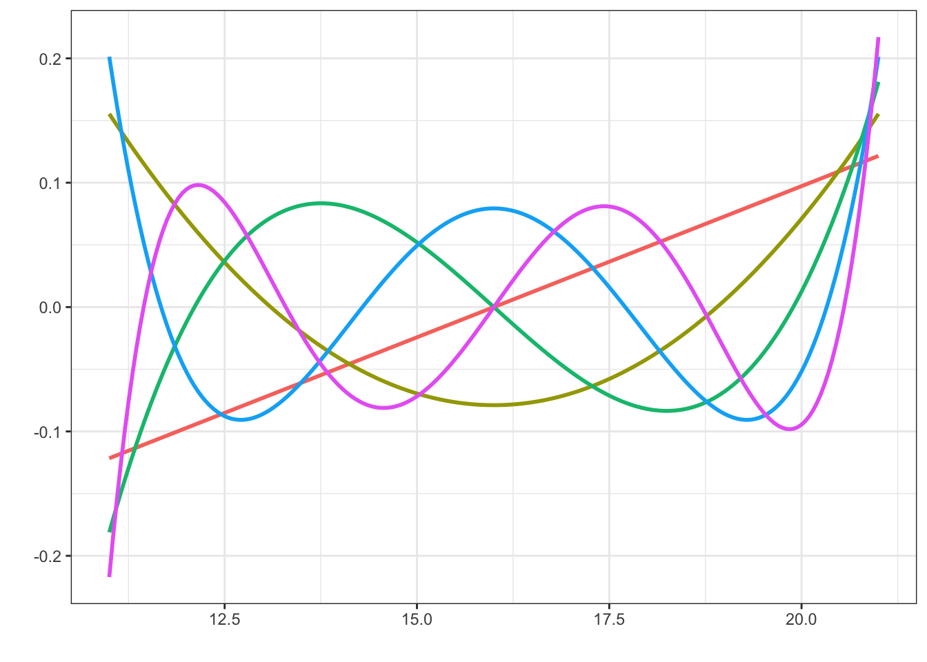
An alternative to data transformations is to use a small but flexible class of basis functions, which can capture the nonlinearity. One possibility is to use low degree polynomials. This can be done by simply including powers of a predictor as additional predictors. [Due to the parsing of formulas in R, powers have to be wrapped into an I()}-call, e.g., y ~ x + I(x2).] Depending on the scale and range of the predictor, this may work just fine. However, raw powers can result in numerical difficulties. An alternative is to use orthogonal polynomials, which are numerically more well behaved.
Figure 2.6 shows an example of an orthogonal basis of degree 5 polynomials on the range 11–21. This corresponds approximately to the range of log(sum), which is a target for basis expansion in the example. What should be noted in Figure 2.6 is that the behavior near the boundary is quite erratic. This is characteristic for polynomial bases. To achieve flexibility in the central part of the range, the polynomials become erratic close to the boundaries. Extrapolation beyond the boundaries cannot be trusted.
An alternative to polynomials is splines. A spline3 is piecewisely a polynomial, and the pieces are joined together in a sufficiently smooth way. The points where the polynomials are joined together are called knots. The flexibility of a spline is determined by the number and placement of the knots and the degree of the polynomials. A degree \(k\) spline is required to be \(k-1\) times continuously differentiable. A degree 3 spline, also known as a cubic spline, is a popular choice, which thus has a continuous (piecewise linear) second derivative.
3 A spline is also a thin and flexible wood or metal strip used for smooth curve drawing.
Code
b_spline <- as_tibble(cbind(x, splines::bs(x, knots = c(14, 18))))
long_b_spline <- tidyr::pivot_longer(b_spline, cols = !x, names_to = "basis_fct")
p + geom_line(data = long_b_spline, linewidth = 1) +
    geom_rug(aes(x = c(11, 14, 18, 21), y = NULL, color = NULL), linewidth = 1)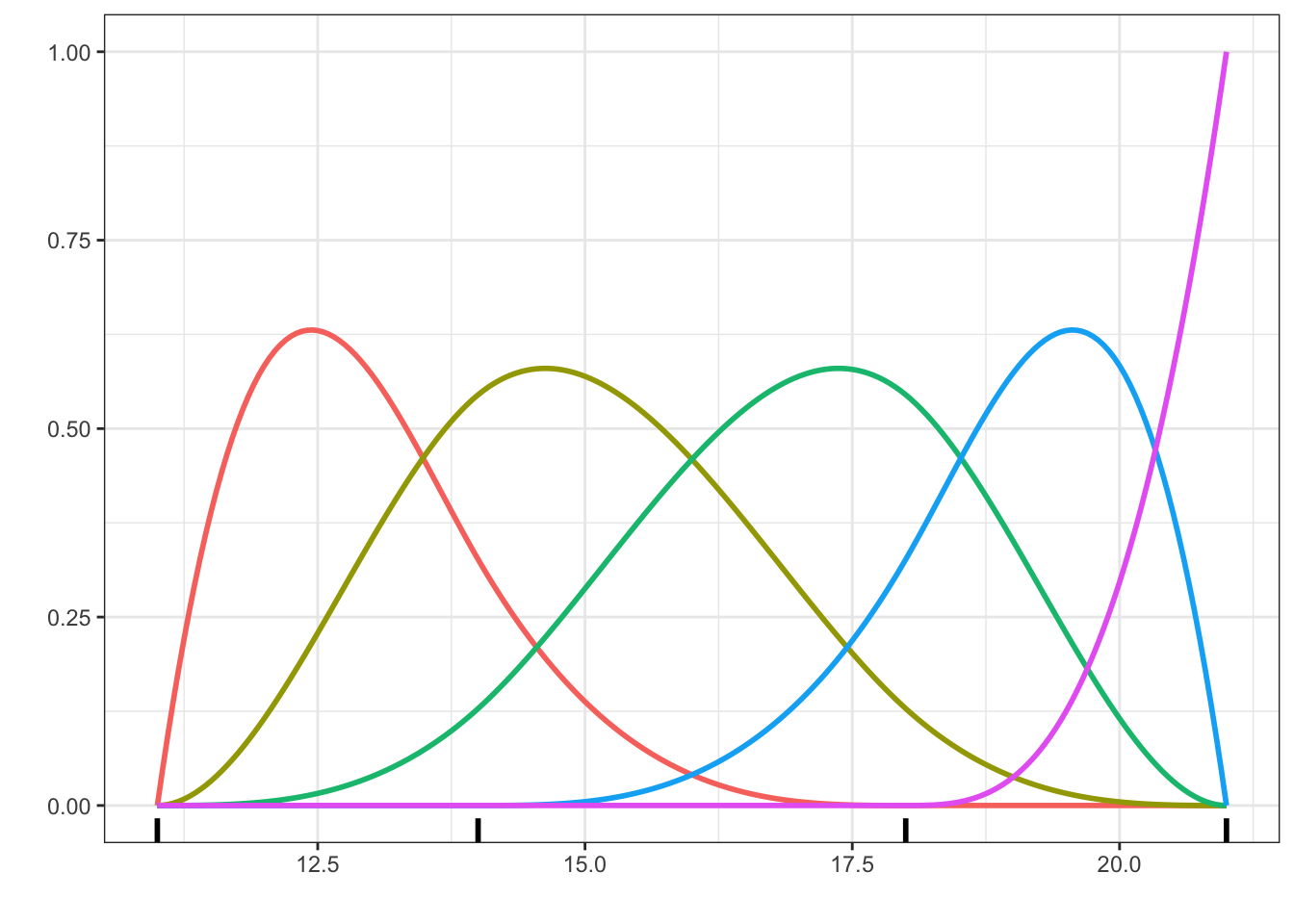
bs() function with two internal knots at 14 and 18 in addition to two boundary knots at 11 and 21.
Figure 2.7 shows a basis of 5 cubic spline functions. They are so-called \(B\)-splines (basis splines). Note that it is impossible to visually detect the knots where the second derivative is non-differentiable. The degree \(k\) \(B\)-spline basis with \(r\) internal knots has \(k + r\) basis functions. The constant function is not included then, and this is precisely what we want when the basis expansion is used in a regression model including an intercept. As seen in Figure 2.7, the \(B\)-spline basis is also somewhat erratic close to the boundary. For a cubic spline, the behavior close to the boundary can be controlled by requiring that the second and third derivatives are \(0\) at the boundary knots. The result is known as a natural cubic spline. The extrapolation (as a spline) of a natural cubic spline beyond the boundary knots is linear.
Due to the restriction on the derivatives of a natural cubic spline, the basis with \(r\) internal knots has \(r + 1\) basis functions. Thus the basis for the natural cubic splines with \(r + 2\) internal knots has the same number of basis functions as the raw cubic \(B\)-spline basis with \(r\) internal knots. This means in practice that, compared to using raw \(B\)-splines with \(r\) internal knots, we can add two internal knots, and thus increase the central flexibility of the model, while retaining its complexity in terms of \(r + 3\) parameters.
Code
n_spline <- as_tibble(cbind(x, splines::ns(x, knots = c(13, 15, 17, 19))))
long_n_spline <- tidyr::pivot_longer(n_spline, cols = !x, names_to = "basis_fct")
p + geom_line(data = long_n_spline, linewidth = 1) +
    geom_rug(aes(x = c(11, 13, 15, 17, 19, 21), y = NULL, color = NULL), linewidth = 1)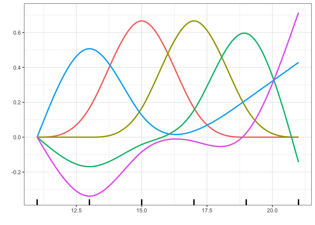
ns() function with internal knots at 13, 15, 17 and 19 in addition to the two boundary knots at 11 and 21.
It is possible to use orthogonal polynomial expansions as well as spline expansions in R together with the lm() function via the functions poly(), bs() and ns(). The latter two are in the splines package, which thus has to be loaded.
We will illustrate the usage of basis expansions for claim size modeling using natural cubic splines.
Code
claims_lm_spline_add <- lm(
  log(claims) ~ ns(log(sum), knots = c(13, 15, 17, 19)) + grp,
  data = claims
)
claims_lm_spline_int <- lm(
  log(claims) ~ ns(log(sum), knots = c(13, 15, 17, 19)) * grp,
  data = claims
)
When we fit a model using basis expansions the coefficients of individual basis functions are rarely interpretable or of interest. Thus reporting the summary including all the estimated coefficients is not particularly informative. Below we only extract the last lines from the summary to report the residual variance and the \(R^2\) quantities.
Code
glance(claims_lm_spline_add) |>
knitr::kable()| r.squared | adj.r.squared | sigma | statistic | p.value | df | logLik | AIC | BIC | deviance | df.residual | nobs |
|---|---|---|---|---|---|---|---|---|---|---|---|
| 0.06416 | 0.0623 | 1.9185 | 34.509 | 0 | 8 | -8352 | 16724 | 16787 | 14822 | 4027 | 4036 |
Code
glance(claims_lm_spline_int) |>
knitr::kable()| r.squared | adj.r.squared | sigma | statistic | p.value | df | logLik | AIC | BIC | deviance | df.residual | nobs |
|---|---|---|---|---|---|---|---|---|---|---|---|
| 0.07294 | 0.06762 | 1.9131 | 13.724 | 0 | 23 | -8333 | 16716 | 16874 | 14683 | 4012 | 4036 |
Compared to the additive model without the basis expansion, \(R^2\) (also the adjusted one) is increased a little by the basis expansion. A further increase is observed for the model that includes interactions as well as a basis expansion, and thus gives a unique nonlinear relation between insurance sum and claim size for each trade group. Figure 2.9 shows some diagnostic plots for the additive model, which show that the mean value model is now pretty good, while the residuals are still slightly right skewed. The lack of normality is not a problem for using the sampling distributions to draw inference. However, if we compute prediction intervals, say, then we must account for the skewness in the residual distribution. This can be done by using quantiles for the empirical distribution of the residuals instead of quantiles for the normal distribution.
Code
claims_diag_spline <- augment(claims_lm_spline_add) ## Residuals etc.
gridExtra::grid.arrange(
  ggplot(claims_diag_spline, aes(.fitted, .resid), alpha = 0.2) + geom_point() + geom_smooth(),
  ggplot(claims_diag_spline, aes(.resid)) + geom_histogram(bins = 40),
  ggplot(claims_diag_spline, aes(sample = .std.resid)) + geom_qq() + geom_abline(),
  ncol = 3
)
Graphical comparisons are typically preferable over parameter comparisons when models involving nonlinear effects and basis expansions are compared.
Code
pred_add <- cbind(
    claims,
    exp(predict(claims_lm_spline_add, interval = "confidence"))
)
pred_int <- cbind(
    claims,
    exp(predict(claims_lm_spline_int, interval = "confidence"))
)
p0 <- p0 + facet_wrap(~ grp, ncol = 4) + coord_cartesian(ylim = c(100, 1e6))
p0 + geom_line(aes(y = fit), pred_add, color = "blue", linewidth = 2) +
  geom_ribbon(aes(ymax = upr, ymin = lwr), pred_add, fill = "blue", alpha = 0.2) +
  geom_line(aes(y = fit), pred_int, color = "red", linewidth = 2) +
  geom_ribbon(aes(ymax = upr, ymin = lwr), pred_int, fill = "red", alpha = 0.2)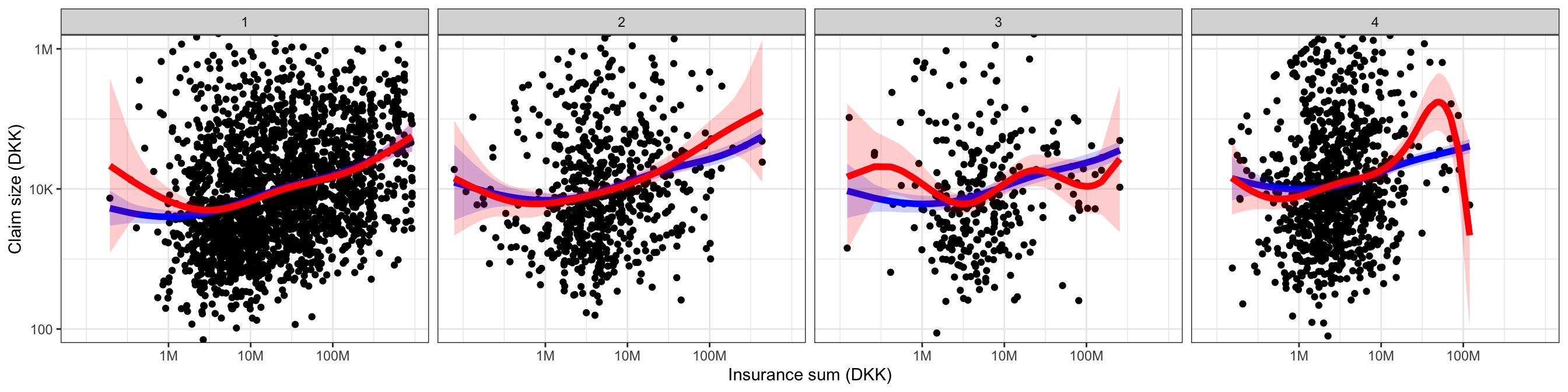
Figure 3.13 shows the fitted models stratified according to trade group. The fitted values were computed using the predict() function in R, which can also give upper and lower confidence bounds on the fitted values. The fitted value for the \(i\)-th observation is \(X_i^T \hat{\beta}\). By Theorem 2.3 a confidence interval for the fitted value can be computed using Equation 2.11 with \(a = X_i\). The confidence intervals reported by predict() for lm objects are computed using this formula, and these are the pointwise confidence bands shown in Figure 3.13. From this figure any gain of the interaction model over the additive model is questionable. The increase of \(R^2\), say, appears to be mostly driven by spurious fluctuations. For trade group 4 the capped claims seem overly influential, and because trade group 3 has relatively few observations the nonlinear fit is poorly determined for this group.
Code
anova(
    claims_lm_add,
    claims_lm_spline_add,
    claims_lm_spline_int
) |> knitr::kable()| Res.Df | RSS | Df | Sum of Sq | F | Pr(>F) |
|---|---|---|---|---|---|
| 4031 | 14902.71 | NA | NA | NA | NA |
| 4027 | 14822.42 | 4 | 80.28605 | 5.484225 | 0.0002115 |
| 4012 | 14683.37 | 15 | 139.04900 | 2.532863 | 0.0009413 |
In the final comparison above using \(F\)-tests we first test the hypothesis that the relation is linear in the additive model, and then we test the additive hypothesis when the nonlinear relation is included. The tests formally reject both hypotheses, but the graphical summary in Figure 3.13 suggests that the nonlinear additive model is preferable anyway.
Introducing a penalty can dampen the spurious fluctuations the arose from the nonlinear basis expansion. We conclude the analysis of the insurance data by illustrating how the penalized least squares fit can be computed, and what effect the penalty has on the least squares solution. First recall that the least squares estimator could have been computed by solving the normal equation directly.
Code
X <- model.matrix(claims_lm_spline_int)
y <- model.response(model.frame(claims_lm_spline_int))
XtX <- crossprod(X)     # Faster than but equivalent to t(X) %*% X
Xty <- crossprod(X, y)  # Faster than but equivalent to t(X) %*% y
coef_hat <- solve(XtX, Xty)
# Comparison
range(coef_hat - coefficients(claims_lm_spline_int))
[1] -1.125585e-09 7.045786e-11The result obtained by solving the normal equation directly is up to numerical errors identical to the solution computed using lm(). The R function solve() calls the Fortran routine DGESV from the LAPACK library for solution of linear equations using LU decomposition with partial pivoting (Gaussian elimination with row permutations).
Likewise, we can compute the penalized estimator by solving the corresponding linear equation. We will do so where we only add a penalty on the coefficients corresponding to the interaction terms in the nonlinear basis expansion. We will use penalty matrices of the form \(\lambda \boldsymbol{\Omega}\) for a fixed matrix \(\boldsymbol{\Omega}\) so that the amount of penalization is controlled by the parameter \(\lambda > 0\).
Code
Omega <- diag(c(rep(0, 9), rep(1, 15)))
coef_hat <- cbind(
solve(XtX + 0.1 * Omega, Xty), # Small penalty
solve(XtX + Omega, Xty), # Medium penalty
solve(XtX + 10 * Omega, Xty) # Large penalty
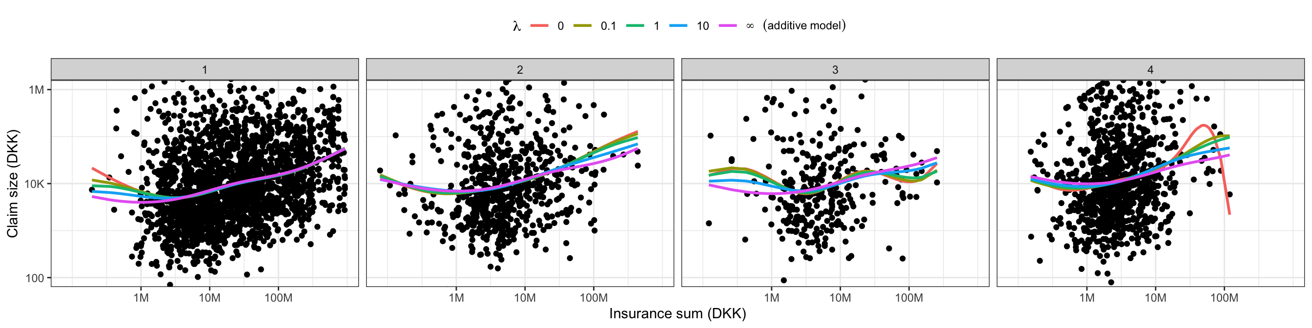
) Figure 2.11 shows the resulting penalized model compared to the unpenalized interaction model (\(\lambda = 0\)) and the additive model (\(\lambda = \infty\)). A minimal penalization is enough to dampen the most pronounced spurious fluctuation for the fourth trade group considerably.
Code
tmp <- cbind(
    coefficients(claims_lm_spline_int),
    coef_hat,
    c(coefficients(claims_lm_spline_add), rep(0, 15))
)
pred <- cbind(claims[, c("sum", "grp")], exp(X %*% tmp))
pred <- tidyr::pivot_longer(pred, cols = !c(grp, sum), names_to = "lambda")
p0 + geom_line(
  aes(y = value, color = lambda),
  data = pred,
  linewidth = 1) +
  theme(legend.position = "top") +
  scale_color_discrete(
    expression(~lambda),
    labels = c(0, 0.1, 1, 10, expression(infinity~~~(additive~model)))
) 
The penalized least squares estimates can also be computed using the QR decomposition via the function lm.fit(). To achieve this we need to augment the model matrix and the response data suitably.
Code
fit_lamb1 <- lm.fit(rbind(X, sqrt(0.1) * Omega), c(y, rep(0, ncol(Omega))))
fit_lamb2 <- lm.fit(rbind(X, sqrt(10) * Omega),  c(y, rep(0, ncol(Omega))))
## Comparisons
range(coef_hat[, 1] - coefficients(fit_lamb1))
[1] -1.621947e-11 2.009581e-11Code
range(coef_hat[, 3] - coefficients(fit_lamb2)) [1] -2.994938e-12 6.206813e-12The results are again (numerically) identical to using solve() above. If several penalized estimates using matrices \(\lambda \boldsymbol{\Omega}\) for different choices of \(\lambda\) are to be computed, a third option using a diagonalization of \(\mathbf{X}^T \mathbf{X}\) is beneficial. This is implemented in, e.g., the lm.ridge() function in the package MASS, which unfortunately doesn’t let you choose your own penalty matrix – it only implements \(\boldsymbol{\Omega} = I\).
In conclusion, we have found evidence in the data for an overall nonlinear relation between insurance sum and claim size plus an additive effect of trade group. For small insurance sums (less than DKK 1M) there is almost no relation, while for larger insurance sums there is roughly a linear relation on a log-log scale. The model fits the data well with a non-normal and slightly right skewed residual distribution, but as a predictive model it is weak, and insurance sum can together with trade group only explain 6-7% of the variation in the (log) claim size distribution.
Exercises
Exercise 2.1 This exercise covers the relation between the formula interface, used to specify a linear model via the lm() function, and the model matrix \(\mathbf{X}\) that a formula generates internally. The formula interface is convenient as it allows us to focus on variables instead of how they are encoded as columns in \(\mathbf{X}\). It is, however, useful to know precisely how R interprets the formulas and translates them into matrices. The lm() function calls the function model.matrix() to create the model matrix from the formula and the data. We usually don’t call this function ourselves, but understanding how it works gives some insight on how exactly formulas are parsed.
We simulate an example dataset to work with. Figure 2.12 shows the simulated data.
Code
set.seed(04022016)
c <- rep(c("A", "B", "C"), each = 50)
formula_data <- tibble(
    x =  rnorm(150, 0),
    z = factor(sample(c)),
    mu = (z == "A") + cos(x) + 0.5 * (z == "B") * sin(x),
    y = rnorm(150, mu, 0.5)
)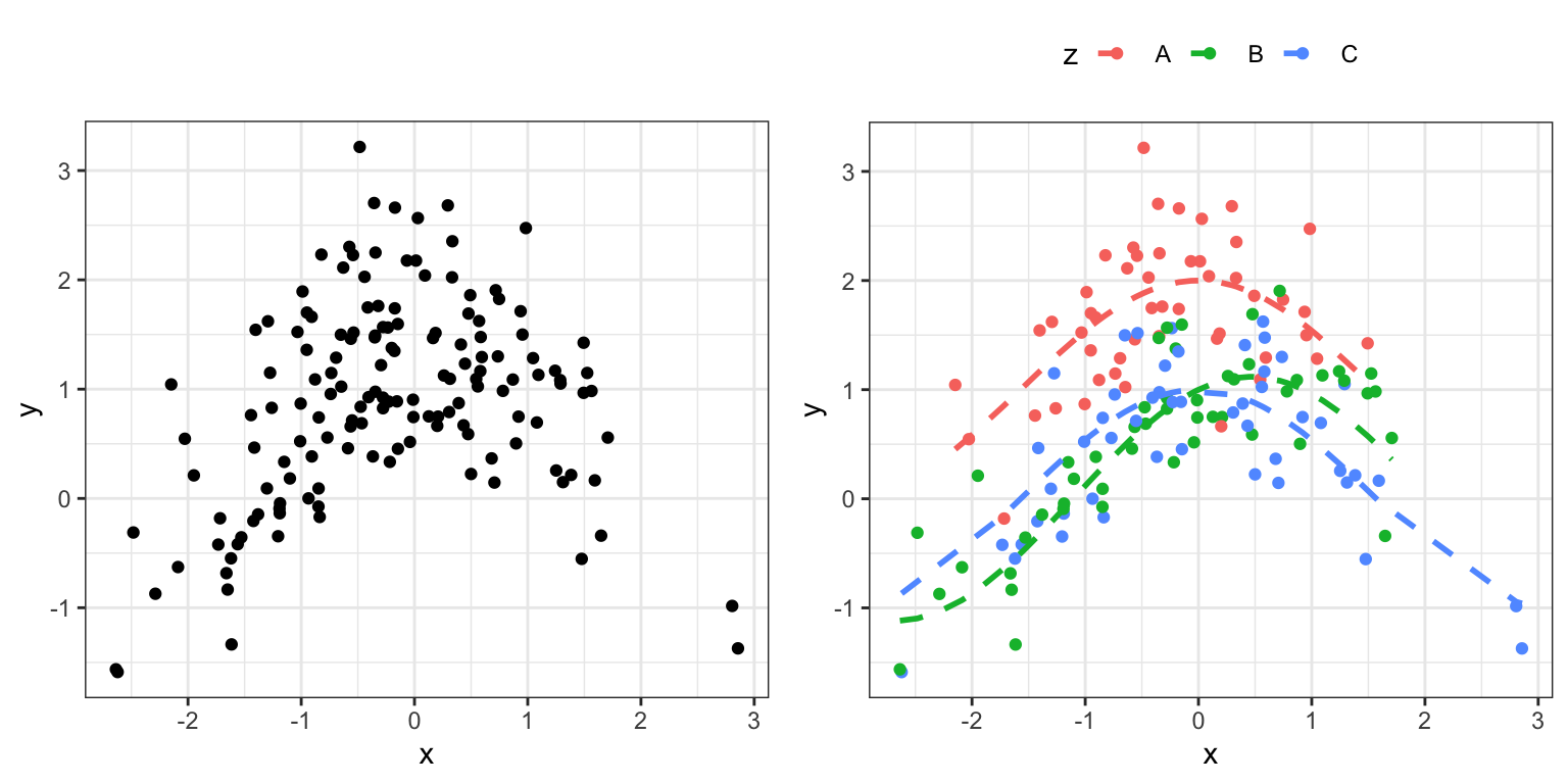
a variable against the b variable. The left figure adds color coding according to the group as encoded by the c variable. The dashed curves are the true means within the three groups.
- Fit a linear regression model using
lm(y ~ x, formula_data)whereyis the response variable andxis the predictor variable. Investigate the residuals. Does the model fit the data?
The formula y ~ x was used internally for the construction of a model matrix with two columns. A column of ones representing the intercept, and a column with the observed values of the predictor variable.
Code
model.matrix(y ~ x, formula_data) |>
    head()
(Intercept) x
1 1 -0.00976291
2 1 -1.64998340
3 1 -0.32014201
4 1 -1.42256848
5 1 1.24188519
6 1 1.08065770- How do you get rid of the intercept via the formula specification?
If we “add a factor” on the right hand side of the formula, e.g., y ~ x + z, the factor’s categorical levels will be represented via dummy variable encodings. If it has \(k\) levels the model matrix gets \(k-1\) additional columns.
Code
model.matrix(y ~ x + z, formula_data) |>
    head()
(Intercept) x zB zC
1 1 -0.00976291 1 0
2 1 -1.64998340 1 0
3 1 -0.32014201 0 0
4 1 -1.42256848 0 1
5 1 1.24188519 1 0
6 1 1.08065770 0 1The precise encoding is controlled by the contrasts.arg argument to model.matrix() (the contrasts argument to lm()) or by setting the contrasts associated with a factor. We can change the base level of z to be level 3 (value C), say.
Code
contrasts(formula_data$z) <-
    contr.treatment(levels(formula_data$z), base = 3)
model.matrix(y ~ x + z, formula_data) |>
    head()
(Intercept) x zA zB
1 1 -0.00976291 0 1
2 1 -1.64998340 0 1
3 1 -0.32014201 1 0
4 1 -1.42256848 0 0
5 1 1.24188519 0 1
6 1 1.08065770 0 0A change of the dummy variable encoding does not change the model (the column space) only the parametrization. This may occasionally be useful for interpretation or for testing certain hypotheses.
- How can you check (numerically) that the two model matrices above span the same column space?
In formulas, the arithmetic operators * and ^ together with : have special meanings.
- Usage of
b * cis equivalent tob + c + b : c. - Usage of
b : cformulates an interaction. - Usage of
(a + b + c)^2is equivalent to(a + b + c) * (a + b + c), which is equivalent toa + b + c + a : b + a : c + b : c, etc.
The following two formulas generate two different model matrices.
Code
model.matrix(y ~ z + x : z, formula_data) |>
    head()
(Intercept) zA zB zA:x zB:x zC:x
1 1 0 1 0.000000 -0.00976291 0.000000
2 1 0 1 0.000000 -1.64998340 0.000000
3 1 1 0 -0.320142 0.00000000 0.000000
4 1 0 0 0.000000 0.00000000 -1.422568
5 1 0 1 0.000000 1.24188519 0.000000
6 1 0 0 0.000000 0.00000000 1.080658Code
model.matrix(y ~ x * z, formula_data) |>
    head()
(Intercept) x zA zB x:zA x:zB
1 1 -0.00976291 0 1 0.000000 -0.00976291
2 1 -1.64998340 0 1 0.000000 -1.64998340
3 1 -0.32014201 1 0 -0.320142 0.00000000
4 1 -1.42256848 0 0 0.000000 0.00000000
5 1 1.24188519 0 1 0.000000 1.24188519
6 1 1.08065770 0 0 0.000000 0.00000000- Are the two models above identical? That is, do the columns of the two model matrices span the same column space?
Transformations of predictor variables can be achieved by formally applying an R function to a variable in the formula specification. Expansions can be achieved by applying an R function that returns a matrix of basis function evaluations when applied to a vector of predictor values. We consider a spline basis expansion.
Code
library(splines)
model.matrix(y ~ ns(x, df = 4), formula_data) |>
    head()
(Intercept) ns(x, df = 4)1 ns(x, df = 4)2 ns(x, df = 4)3 ns(x, df = 4)4
1 1 0.75361809 0.169569207 0.08775628 -0.04862859
2 1 0.07603605 -0.191091633 0.44504011 -0.25394848
3 1 0.77817043 0.005536704 0.13653515 -0.07790959
4 1 0.14168625 -0.207697339 0.48371373 -0.27601639
5 1 0.15040919 0.515081509 0.26234462 0.07216468
6 1 0.20011297 0.527404800 0.24317864 0.02930359Before you run the R expression below, answer the following question on the basis of what you have learned.
- Determine the number of columns for the model matrix below and explain and interpret what the columns mean?
Code
model.matrix(y ~ ns(x, df = 4) * z, formula_data) |>
    head()
Figure 2.13 was obtained by fitting the linear model using the model matrix, or rather the formula, from above. The figure illustrates the model fit by comparing the fitted model directly to the true means and via the residuals. Fitted values and residuals were computed using the augment() function from the broom package.
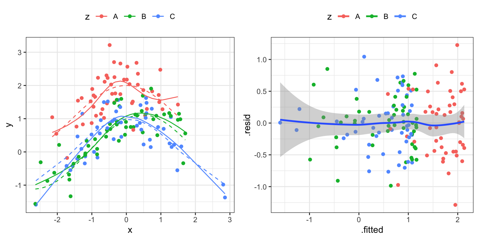
- Reproduce Figure 2.13 and discuss the model fit.
Exercise 2.2 This exercise is based on a dataset relating the mean verbal SAT scores for each of the 50 US states to the percentage of students taking the test. The data comes with the RwR package.
Code
library(RwR)
data(sat, package = "RwR")
Fit a linear regression model (with an intercept) of the state SAT score as a function of percentage of students. Add the fitted line to the plot.
Fit a piecewise affine function with the “bend” at 50% of the students taking the test. How can you formally test the linearity assumption in Question 1 within this larger model?
Hint: you want to fit a linear model with a model matrix \(\mathbf{X}\) with 3 columns representing an intercept and two piecewise linear functions. You can, for instance, generate a basis using an
ifelse()construction in the formula. Try different bases. Is there anyone particularly suitable for testing the linearity assumption?Fit a natural cubic spline model with 4 knots. Use the
ns()function to generate a B-spline basis. How should you choose the placements of the knots? How can you formally test the linearity assumption within this larger model?
Exercise 2.3 Show that if (2.13) holds then \[C = (\mathbf{X}^T \mathbf{X})^{-1} \mathbf{X}^T \mathbf{X}'.\] Explain how this can be used to check if the column space of an arbitrary \(\mathbf{X}'\) is contained in the column space of \(\mathbf{X}\).
Exercise 2.4 Consider the following matrices
X <- splines::bs(
    seq(0, 1, 0.01),
    knots = c(0.3, 0.5, 0.7)
)
X_prime <- seq(0, 1, 0.01)
of \(B\)-spline basis functions evaluated on a grid in the interval \([0, 1]\). Use the previous exercise to verify that X_prime is in the column space of X. You can use the formula from the exercise to compute \(C.\) Can you also use lm.fit()?
Exercise 2.5 Let \(C\) be any \(n \times p\) matrix and consider the linear estimator \[ \tilde{\beta} = C^T \mathbf{Y}. \]
- Show that \(\tilde{\beta}\) is unbiased as an estimator of \(\beta\) if A1 and A4 hold and if \[\beta = C^T \mathbf{X} \beta\] for all \(\beta\).
- Show that if the estimator is unbiased and A1, A2 and A4 hold then \[V(\tilde{\beta} \mid \mathbf{X}) = \sigma^2 C^TC\] and that \[V(\hat{\beta}- \tilde{\beta} \mid \mathbf{X}) = \sigma^2 (C^TC - (\mathbf{X}^T\mathbf{X})^{-1})\] where \(\hat{\beta}\) is the least squares estimator.
- Explain that this shows the Gauss-Markov theorem: Under the assumptions A1 + A2 + A4 the least squares estimator of \(\beta\) has minimal variance among all linear, unbiased estimators of \(\beta\).
Exercise 2.6 This exercise relates the empirical correlations between the predictor variables to the variance of the least squares estimator. The setup is as follows. The matrix \(\mathbf{X}\) denotes an \(n \times p\) matrix of predictor variables, \(\mathbf{1}\) denotes an \(n\) dimensional column vector of ones and \((\mathbf{1} \ \ \mathbf{X})\) denotes the \(n \times (p+1)\) matrix with the first column being \(\mathbf{1}\) and the remaining \(n \times p\) block being \(\mathbf{X}\). We let \[\bar{X} = \frac{1}{n} \mathbf{X}^T \mathbf{1}\] denote the \(p\) dimensional vector of mean values for the predictor, and we let \[\hat{\Sigma} = \frac{1}{n} (\mathbf{X} - \mathbf{1} \bar{X}^T)^T (\mathbf{X} - \mathbf{1} \bar{X}^T)\] denote the empirical covariance matrix. It is assumed that \(\hat{\Sigma}\) is invertible.
- Show that \[ n \hat{\Sigma} = \mathbf{X}^T \mathbf{X} - n \bar{X} \bar{X}^T. \]
- Use block matrix inversion to show that \[ \Big((\mathbf{1} \ \ \mathbf{X})^T (\mathbf{1} \ \ \mathbf{X})\Big)^{-1} = \left(\begin{array}{cc} * & * \\ * & \frac{1}{n} \hat{\Sigma}^{-1} \end{array} \right). \] Here the \(*\)-s mean some values that we are not interested in computing in this exercise.
- Show that if we fit a linear model with an intercept (which is denoted \(\beta_0\)) using the least squares estimator, then the variance of \(\hat{\beta}_i\), conditionally on \(\mathbf{X}\), for \(i = 1,\ldots, p\) is \[ \frac{\sigma^2}{n} \left(\hat{\Sigma}^{-1}\right)_{ii}. \]
With \(\hat{\Sigma}_{-1}\) denoting the empirical covariance matrix with the first row and column removed we can write \(\hat{\Sigma}\) in block form as \[ \hat{\Sigma} = \left( \begin{array}{cc} \hat{\sigma}_1^2 & \hat{\gamma}^T \\ \hat{\gamma} & \hat{\Sigma}_{-1} \end{array} \right). \]
- Use block inversion (again) to show that \[ \left(\hat{\Sigma}^{-1}\right)_{11} = \frac{1}{\hat{\sigma}_1^2 - \hat{\gamma}^T \left(\hat{\Sigma}_{-1}\right)^{-1} \hat{\gamma}}. \]
- Show that in the case \(p = 2\), the formula above reduces to \[ \left(\hat{\Sigma}^{-1}\right)_{11} = \frac{1}{\hat{\sigma}_1^2 (1 - \widehat{\text{corr}}(X_1, X_2)^2)}. \]
- Show that if \(\mathbf{X}_{\cdot 1} - \mathbf{1} \bar{X}_1\) is perpendicular to the remaining columns in \(\mathbf{X} - \mathbf{1}\bar{X}^T\), then \[ \left(\hat{\Sigma}^{-1}\right)_{11} = \frac{1}{\hat{\sigma}_1^2}. \]
- Interpret the results obtained in this exercise in terms of how the empirical variance of and empirical correlation between predictor variables affect the variances of the estimators \(\hat{\beta}_i\) for \(i = 1, \ldots, p\).