12  Company default – a case study

Important

This chapter is still a rough draft of a case study on modeling time to company default using survival modeling techniques. For now it will not be substantially revised.

12.1 Outline and prerequisites

This chapter is based on a dataset collected by the winners of a competition (Business Analytics Challenge, 2017). The data considered in this chapter is a subset of the full dataset. It contains some key financial variables from the annual reports of Danish companies from the period 2013 to 2016. The dataset also contains information about whether the companies defaulted during the time period. Our objective is to build a predictive model of the time until default of a company and use this model to explore the associations between the various financial predictors and this survival distribution of the company.

The chapter primarily relies on the following R packages.

library(RwR)
library(ggplot2)
library(tibble)
library(tidyr)
library(skimr)
library(lubridate)
library(broom)
library(splines)
library(dplyr)
library(survival)

12.2 Exploratory analysis

In this section we load the data and present some aspects of the dataset. We reorganize and clean the data to bring the data on a form where it is suitable for modeling the survival distribution of companies.

data(default, package = "RwR")

The first nine rows of the dataset.

fiscal_start	fiscal_end	default	equity	profit	assets	return_on_assets	CVR	start	end	industry_type	econ_activity	competition_density
2013-01-01	2013-12-31	0	39217	-76713	56399	-1.3601837	10000025	2012-05-31	NA	Andre serviceydelser mv.	117783.52	11.90596
2014-01-01	2014-12-31	0	-798210	-47427	357316	-0.1327313	10000025	2012-05-31	NA	Andre serviceydelser mv.	119485.02	16.45823
2015-01-01	2015-12-31	0	-972885	-174675	389334	-0.4486508	10000025	2012-05-31	NA	Andre serviceydelser mv.	122500.40	23.11156
2013-01-01	2013-12-31	0	67255000	20058000	194020000	0.1033811	10000157	1999-10-14	NA	Finansiering og forsikring	27109.54	39.30419
2014-01-01	2014-12-31	0	96773000	24198000	226974000	0.1066113	10000157	1999-10-14	NA	Finansiering og forsikring	27390.44	47.44786
2015-01-01	2015-12-31	0	112820000	16185000	200219000	0.0808365	10000157	1999-10-14	NA	Finansiering og forsikring	27694.80	72.85417
2014-01-01	2014-12-31	0	694457	128263	739690	0.1734010	10000211	1999-09-29	NA	Finansiering og forsikring	23162.49	46.28104
2013-01-01	2013-12-31	0	566194	58620	942710	0.0621824	10000211	1999-09-29	NA	Finansiering og forsikring	22890.15	37.60334
2015-01-01	2015-12-31	0	764365	69908	804631	0.0868821	10000211	1999-09-29	NA	Finansiering og forsikring	23401.06	69.67308

Each row in the dataset corresponds to an annual report from a Danish company. The dataset was constructed in May, 2017, by extracting annual reports for all Danish companies from the period 2013–2016.

Variables:

• fiscal_start: Start date of fiscal year.
• fiscal_end: End date of fiscal year.
• default: Indicator of whether the company defaulted.
• equity: Equity in DKK from the annual report that fiscal year.
• profit: Profit in DKK from the annual report that fiscal year.
• assets: Assests in DKK from the annual report that fiscal year.
• return_on_assets: The profit / assets (ROA) ratio.
• CVR: The unique Danish company identification number as character.
• start: Registered start date of company.
• end: Registered end date of company. Missing if the company is not registered as closed.
• industry_type: A categorical variable.
• econ_activity: A numerical variable indicating the economic activity in spatial proximity of the company.
• competition_density: A numerical variable indicating the competition in spatial proximity of the company.

We reorganize the data so that each row corresponds to a single company and contains the data from the earliest annual report in the dataset for that company. The end variable is missing if the company was not closed when the data was gathered, and we choose to replace these missing values by the administrative censoring date “2017-05-01”.

default <- group_by(default, CVR) |>
  summarize(fiscal_end = min(fiscal_end, na.rm = TRUE)) |> 
  inner_join(default, y = _) |>
  mutate(end = replace_na(end, as_date("2017-05-01")))

Since the annual report is not publicly available immediately after the end of the fiscal year we decide that the baseline date for the company is five months after the end of the fiscal year. We clean the data by removing all rows where:

• The fiscal year starts after it ends (data error).
• The company is closed within five months after the end of the fiscal year.
• The company has a start date later than the end of the fiscal year.

default <- filter(
    default, 
    fiscal_start < fiscal_end, 
    fiscal_end + months(5) < end, 
    start <= fiscal_end
)

skim(default)

Variable type: character

skim_variable	n_missing	complete_rate	min	max	empty	n_unique	whitespace
CVR	0	1	8	8	0	227204	0
industry_type	37	1	6	29	0	20	0

Variable type: Date

skim_variable	n_missing	complete_rate	min	max	median	n_unique
fiscal_start	0	1	2011-11-29	2016-11-25	2013-03-01	1398
fiscal_end	0	1	2012-12-31	2016-11-30	2013-12-31	194
start	0	1	1735-06-10	2016-11-25	2007-11-15	14351
end	0	1	2014-01-28	2017-05-17	2017-05-01	910

Variable type: factor

skim_variable	n_missing	complete_rate	ordered	n_unique	top_counts
default	0	1	FALSE	2	0: 217881, 1: 9323

Variable type: numeric

skim_variable	n_missing	complete_rate	mean	sd	p0	p25	p50	p75	p100	hist
equity	1	1.00	25336557.89	1.873027e+09	-7.217768e+10	45314.00	408648.00	2536798.50	7.100090e+11	▇▁▁▁▁
profit	4	1.00	1481978.49	1.698615e+08	-4.249600e+10	-28084.12	26558.50	329493.25	4.093200e+10	▁▁▇▁▁
assets	5503	0.98	55588303.44	5.377255e+09	-3.106368e+06	278214.00	1453551.00	6146500.00	2.397053e+12	▇▁▁▁▁
return_on_assets	14586	0.94	70.20	2.526159e+05	-8.531832e+07	-0.04	0.02	0.13	6.382979e+07	▁▁▇▁▁
econ_activity	10175	0.96	61761.28	4.513554e+04	1.159632e+04	28498.85	38437.84	100475.22	2.012026e+05	▇▂▁▂▁
competition_density	5234	0.98	117.41	2.076000e+02	0.000000e+00	11.25	29.32	97.19	1.208950e+03	▇▁▁▁▁

Table 12.1: Data summary of the default data using the skim() function.

We introduce two new variables.

• age: The age in days of the company at baseline.
• followup: The time from baseline in days and until the company is either closed or administratively censored.

default <- mutate(
    default, 
    age = as.numeric(fiscal_end + months(5) - start),
    followup = as.numeric(end - (fiscal_end + months(5)))
)

We will model followup as the censored survival time until default with the status indicator being default == 1. The baseline is the end of the company’s first fiscal year plus five months. The predictor variables we will use are all available at baseline, and we do, e.g., not use information from subsequent annual reports. Though such information might be informative about the trajectories taken by companies that end up defaulting, we cannot meaningfully use the information as predictors at baseline.

A fraction of companies have missing values of assets and a larger fraction has missing values of return_on_assets. Upon inspection it turns out that return_on_assets is missing if either assets is missing or equal to zero. Below we impute both values as zero if they are missing.

We also note from the summary statistics above that all the financial variables span multiple orders of magnitude. We therefore choose to nonlinearly normalize these variables to bring them on a common scale. This can be done in many ways, e.g., by using the marginal empirical distributions to transform each variable to the unit interval. Below we choose to first standardize variables by the inter-quartile range and then to transform them to the interval \((-1, 1)\) by the (scaled) arctangent function. This handles the heavy tails well and the zero remains interpretable. We finally log-transform age.

# norm <- function(x) rank(x) / length(x) # quantile normalization
# norm <- function(x) atan((x - median(x, na.rm = TRUE)) / IQR(x, na.rm = TRUE))
norm <- function(x) 2 * atan( x / IQR(x, na.rm = TRUE)) / pi
default <- mutate(default,
    assets = replace_na(assets, 0),
    return_on_assets = replace_na(return_on_assets, 0),
    equity_norm = norm(equity),
    assets_norm = norm(assets),
    profit_norm = norm(profit),
    return_norm = norm(return_on_assets), 
    log_age = log10(age)
)

After the normalize and transformation it is meaningful to explore the pairwise associations between the predictor variables, e.g., in terms of the scatter plot matrix in Figure 12.1. The association patterns are complicated for several different reasons. For once, because there are certain logical constraints among the variables (equity and assets, profit and return).

ggally_hexbin <- function(data, mapping, ...) 
    ggplot(data, mapping) + stat_binhex(...) 
ggally_spear <- function(...) GGally::ggally_cor(..., method = "spearman", stars = FALSE)

GGally::ggpairs(
    na.omit(default), 
    columns = c("log_age", "equity_norm", "assets_norm", "profit_norm", "return_norm"), 
    upper = list(continuous = "spear"),
    lower = list(continuous = GGally::wrap("hexbin", bins = 150)), 
) + scale_fill_continuous(trans = "log")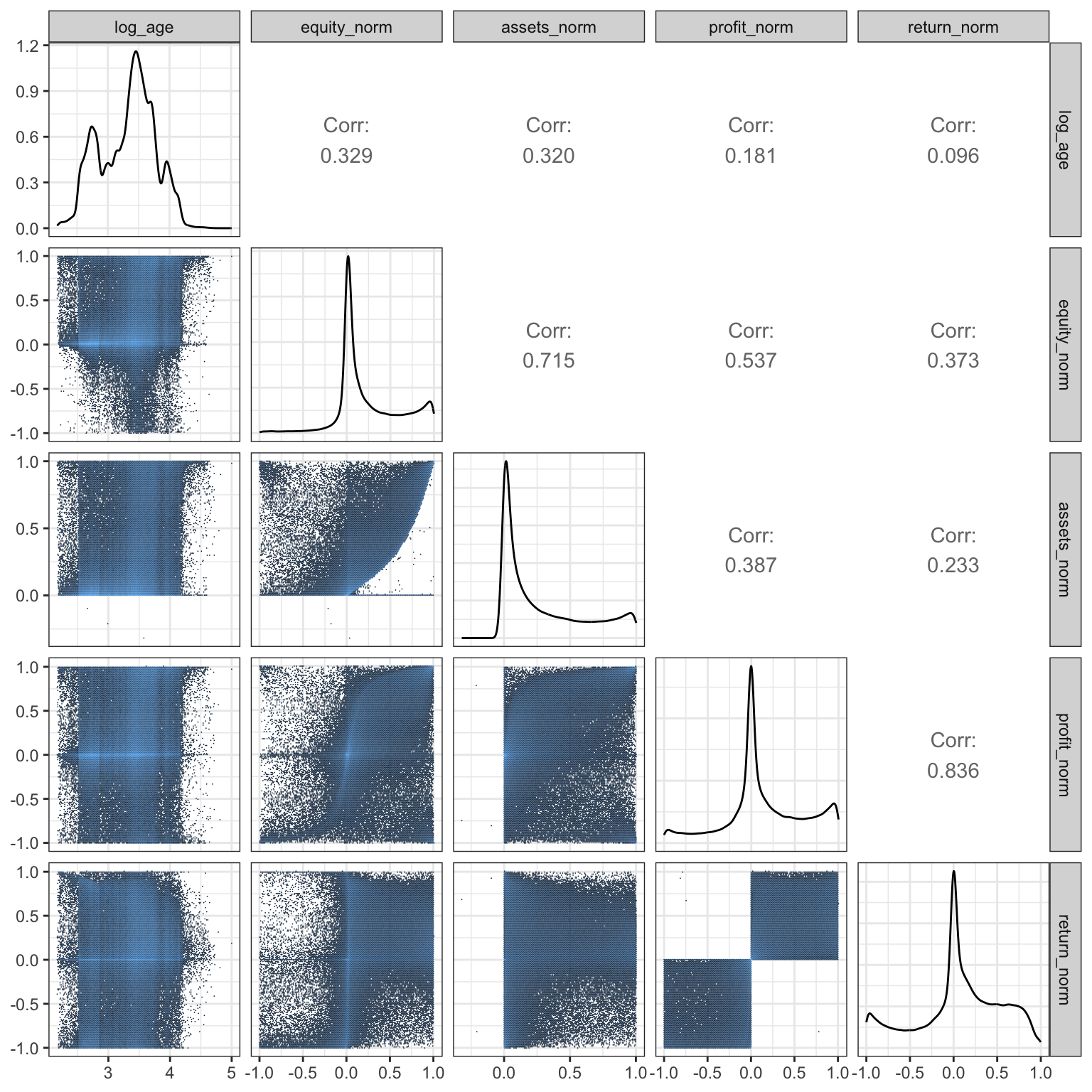 

Figure 12.1: Scatter plot matrix of the normalized numerical variables and corresponding Spearman correlations.

12.3 A Cox model

We illustrate the modeling of company default by fitting a Cox model using an additive model on the log hazard ratio scale using nonlinear spline expansions of the five numerical predictors. We choose to only consider one of the industry types corresponding to about 30000 of the companies.

form <- Surv(followup, default == 1) ~ 
    ns(log_age, df = 5) + ns(equity_norm, df = 5) + ns(assets_norm, df = 5) +
    ns(profit_norm, df = 5) + ns(return_norm, df = 5)
default_trade <- filter(default, industry_type == "Handel")
default_cox <- coxph(form, data = default_trade)

The baseline estimate of the survival function for the Cox model is then computed.

baseline <- survfit(default_cox) |>
        summary(data.frame = TRUE)

ggplot(baseline, aes(time, surv)) + 
        geom_ribbon(aes(ymin = lower, ymax = upper), fill = "gray60", alpha = 0.4) +
        geom_step(color = "#3366FF") +
        ylim(0.8, 1) +
        scale_x_continuous(
            "followup time", 
            breaks = c(0, 365, 2 * 365, 3 * 365), 
            labels = c("baseline", "one year", "two years", "three years")) + 
        ylab("survival probability")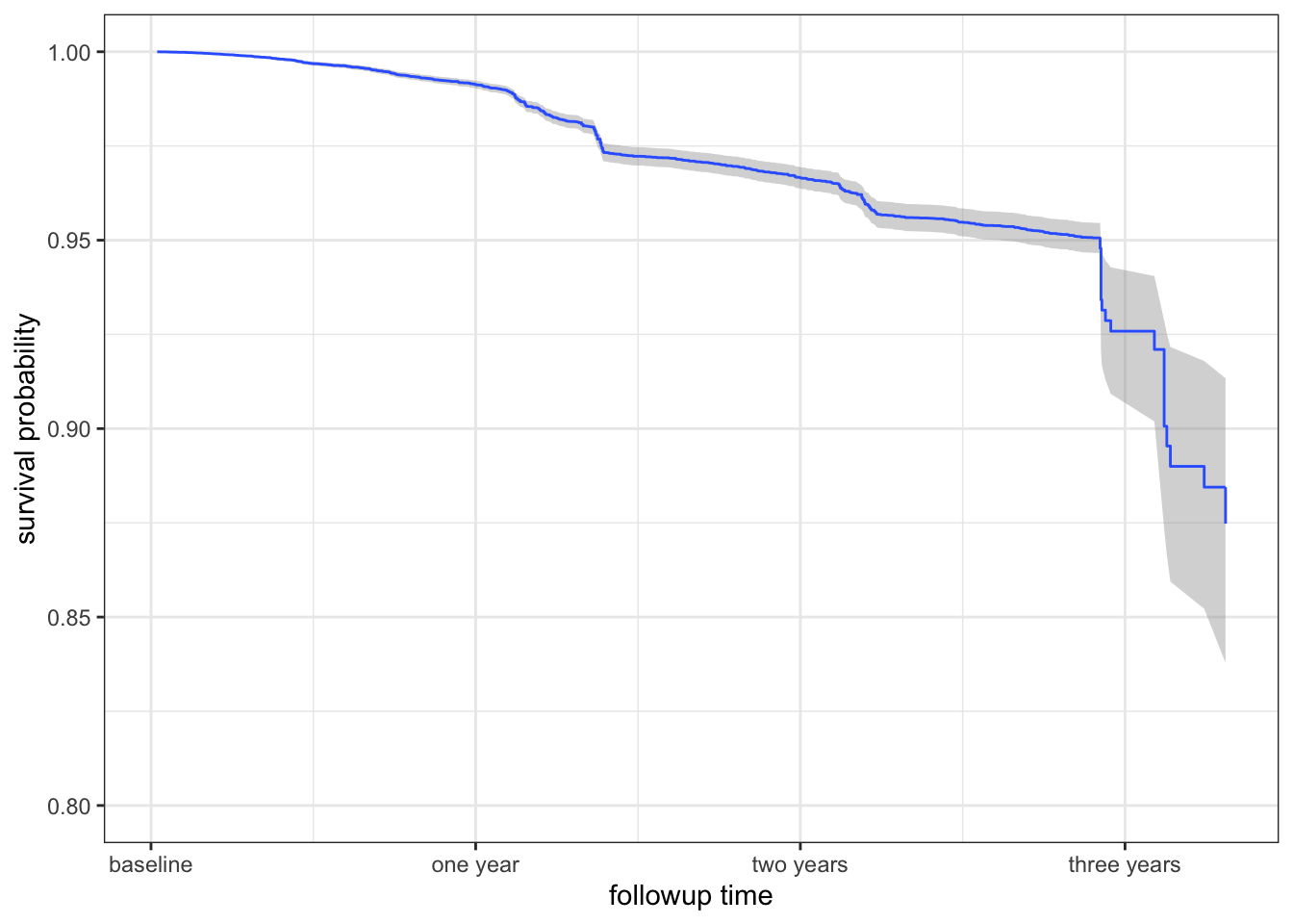 

Baseline survival function for the Cox model of default.

12.3.1 Model predictions

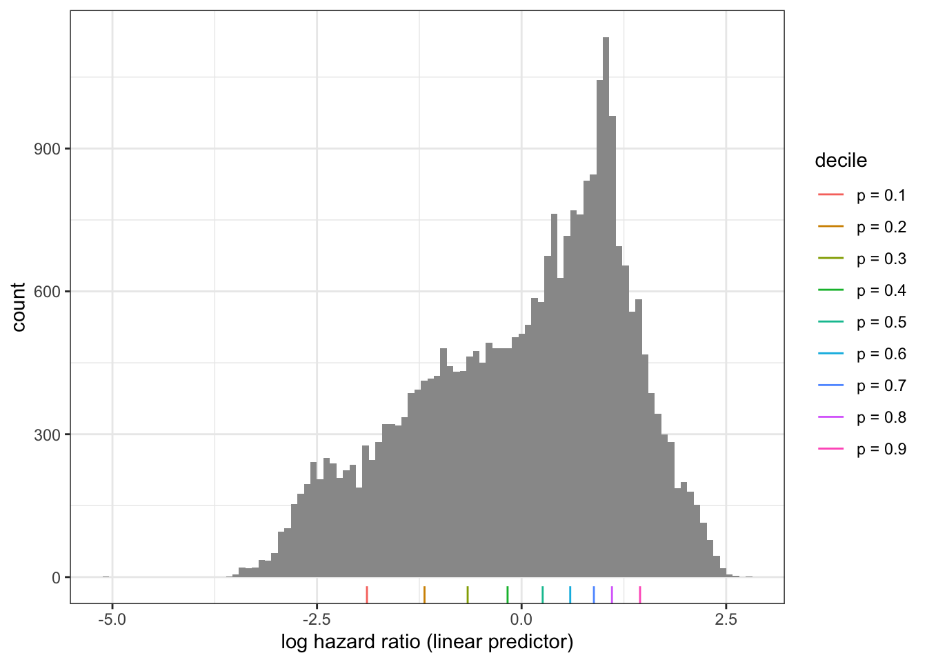
To understand the model better we first explore model predictions. Figure 12.2 shows the empirical distribution of the log hazard ratios on the dataset. Recall that for the proportional hazards model, a log hazard ratio of \(-2.5\) corresponds to a multiplicative effect of \(e^{-2.5} = 0.082 \approx 1/12\) on the (cumulative hazard), while a log hazard ratio of \(2.5\) corresponds to a multiplicative effect of \(e^{2.5} \approx 12\).

default_pred <- predict(default_cox)

probs <- seq(0.1, 0.9, 0.1)
prob_names <- paste("p =", probs)
qt <- quantile(default_pred, probs = probs)
ggplot(mapping = aes(x = default_pred)) + 
    geom_histogram(bins = 100, fill = "gray60") +
    xlab("log hazard ratio (linear predictor)") +
    geom_rug(
        data = tibble(default_pred = qt, decile = prob_names), 
        aes(color = decile), 
        show.legend = TRUE 
    )

Figure 12.2: Distribution of the log hazard ratio (the linear predictor) on the data. The colored marks are the deciles of the distribution.

To visualize the range of predicted survival functions for different companies, depending on their predictors, Figure 12.3 shows the survival curves for the different deciles of the distribution of the log hazard ratios.

baseline_aug <- baseline
for (i in seq_along(probs)) {
    baseline_aug$x = qt[i]
    names(baseline_aug)[ncol(baseline_aug)] <- prob_names[i]
} 
surv_range <- pivot_longer(
    baseline_aug, 
    cols = all_of(prob_names),
    names_to = "decile",
    values_to = "lhr"
    ) |>
    mutate(
        cumhaz = exp(lhr) * cumhaz,
        surv = exp(-cumhaz)
    )

ggplot(surv_range, aes(time, surv, color = decile)) + 
        geom_step() +
        ylim(0.6, 1) +
        scale_color_brewer(palette = "Set1") +
        scale_x_continuous(
            "followup time (years)", 
            breaks = c(0, 365, 2 * 365, 3 * 365), 
            labels = c("baseline", "one year", "two years", "three years")) + 
        ylab("survival probability")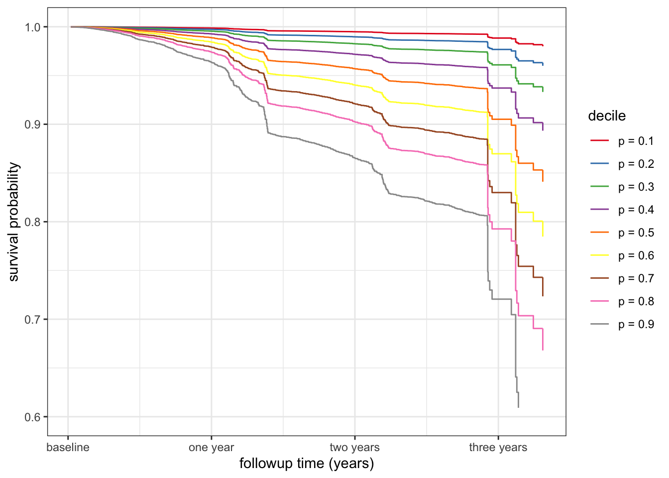 

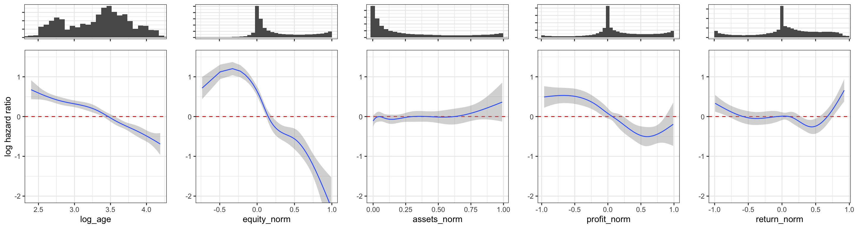
Figure 12.3: Survival functions for the different deciles of the distribution of the log hazard ratio.

We will finally show how each of the individual nonlinear functions in the formula specification are estimated. This can be done using the predict() function specifying type = "terms" to get a prediction for each term in the formula. Figure 12.4 shows the five different functions including a pointwise 95% confidence band based on the standard errors that are also computed by the predict() function.

probs <- seq(0.01, 0.99, 0.01)
pred_frame <- reframe(
    default, 
    log_age = quantile(log_age, probs = probs, na.rm = TRUE),
    equity_norm = quantile(equity_norm, probs = probs, na.rm = TRUE),
    assets_norm = quantile(assets_norm, probs = probs, na.rm = TRUE),
    profit_norm = quantile(profit_norm, probs = probs, na.rm = TRUE),
    return_norm = quantile(return_norm, probs = probs, na.rm = TRUE)
)
pred_default <- predict(
    default_cox, 
    newdata = pred_frame, 
    type = "terms", 
    se.fit = TRUE
)

p <- ggplot(mapping = aes(x, y, ymin = y - 1.96 * se, ymax = y + 1.96 * se)) + 
    geom_hline(yintercept = 0, color = "red", linetype = 2) +
    geom_ribbon(fill = "grey60", alpha = 0.4) + 
    geom_line(color = "#3366FF") + coord_cartesian(ylim = c(-2, 1.5)) + ylab("")

p_bar <- ggplot(default) + geom_histogram(bins = 40) + ylab("") +
    scale_y_continuous(label = \(x) rep("   ", length(x))) +
    theme(
        axis.title.x = element_blank(),
        axis.text.x = element_blank(),
    )

gridExtra::grid.arrange(
p_bar + aes(x = log_age) + coord_cartesian(xlim = range(pred_frame$log_age)),
p_bar + aes(x = equity_norm) + coord_cartesian(xlim = range(pred_frame$equity_norm)),
p_bar + aes(x = assets_norm) + coord_cartesian(xlim = range(pred_frame$assets_norm)), 
p_bar + aes(x = profit_norm) + coord_cartesian(xlim = range(pred_frame$profit_norm)), 
p_bar + aes(x = return_norm) + coord_cartesian(xlim = range(pred_frame$return_norm)),
p %+% tibble(
        x = pred_frame$log_age, 
        y = pred_default[[1]][, 1], se = pred_default[[2]][, 1]
    ) + xlab("log_age") + ylab("log hazard ratio"),
p %+% tibble(
        x = pred_frame$equity_norm, 
        y = pred_default[[1]][, 2], se = pred_default[[2]][, 2]
    ) + xlab("equity_norm"),
p %+% tibble(
        x = pred_frame$assets_norm, 
        y = pred_default[[1]][, 3], se = pred_default[[2]][, 3]
    ) + xlab("assets_norm"),
p %+% tibble(
        x = pred_frame$profit_norm, 
        y = pred_default[[1]][, 4], se = pred_default[[2]][, 4]
    ) + xlab("profit_norm"),
p %+% tibble(
        x = pred_frame$return_norm, 
        y = pred_default[[1]][, 5], se = pred_default[[2]][, 5]
    ) + xlab("return_norm"),
    ncol = 5,
    heights = c(1, 4)
)

Figure 12.4: Term plot for the five spline terms in the Cox model of company default. The blue band is a pointwise 95% confidence band. The histograms above indicate the marginal distributions of the variables in the data.

12.3.2 Model diagnostic

We investigate the model fit using residual plots.

p1 <- augment(default_cox, data = default_trade, type.predict = "expected") |>
    survfit(Surv(.fitted, default == 1) ~ 1, data = _) |>
    summary(data.frame = TRUE) |>
    ggplot(aes(time, cumhaz)) + 
    geom_abline(slope = 1, color = "blue") +
    geom_point(alpha = 0.2) +
    xlab("Cox-Snell residuals") + 
    ylab("Cumulative hazard")

binScale <- scale_fill_continuous(
  breaks = c(1, 10, 100, 1000, 10000),
  low = "gray80", 
  high = "black",
  trans = "log", 
  guide = "none"
)

p2 <- augment(default_cox) |> 
    ggplot(aes(.fitted, .resid)) +
    geom_hex(bins = 200) + 
    binScale + 
    geom_smooth() + 
    xlab("Fitted values") +
    ylab("Martingale residuals") +
    coord_cartesian(xlim = c(-2, 4), ylim = c(-1, 1))

gridExtra::grid.arrange(p1, p2, ncol = 2)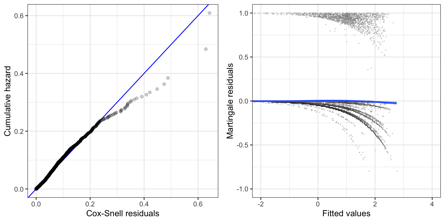

Figure 12.5: Residual diagnostics for the Cox model of default.

Figure 12.5 shows that the Cox model does not fit the data perfectly.

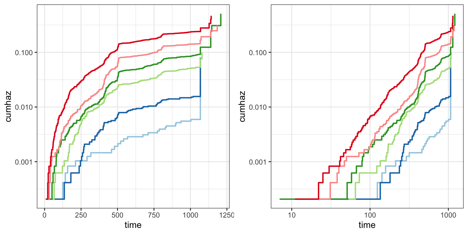
Figure 12.6 investigates the proportional hazards assumption more specifically. It is constructed by stratifying the data according to quantiles of the linear predictor and then fit a nonparametric survival function for each strata. If the proportional hazards assumption holds, the corresponding cumulative hazard functions should be roughly proportional. This is easiest to assess if they are further log-transformed, because on that scale proportionality corresponds to translations.

It is common to also log-transform the time scale (right plot in Figure 12.6). The cumulative hazard function often has the shape of a power function, which on the log-log scale becomes a straight line. Proportionality implies that these lines are roughly vertical translations of each other. Deviations appear in either plot as either direct crossings of the curves or just differences in slope or shape among the curves. In this case there might to be some issues with the proportionality assumption, both when comparing the low risk companies (blue) to the other companies and when comparing the two medium risk groups (green) to each other.

probs <- seq(0, 1, length.out = 7)
qt <- quantile(default_pred, probs = probs)
labels <- paste("p =", cumsum(diff(probs)))
default_trade$eta <- default_pred
default_diag <- survfit(Surv(followup, default == 1) ~ cut(eta, breaks = qt), data = default_trade) |>
    summary(data.frame = TRUE) |> 
    mutate(strata = factor(strata, labels = labels))

p1 <- ggplot(default_diag, aes(time, cumhaz, color = strata)) + 
    geom_step(linewidth = 0.8) + 
    scale_y_log10() +
    scale_color_brewer(palette = "Paired") 

p1 <- p1 + theme(legend.position = "none") 

gridExtra::grid.arrange(p1, p1 + scale_x_log10(), ncol = 2)

Figure 12.6: The log cumulative hazard function fitted to strata based on the quantiles of the linear predictor. In the right plot the time axis is on a log scale.